Tidymodels for omics data: Part 1

Downloading and exploring TCGA (breast cancer) expression data from GEO so we can proceed to use machine learning later. We’ll also make some exploratory plots such as survival analysis

Author

Mark Dunning

Published

November 11, 2025

Pre-amble

This will be the first in a series where I look at machine learning techniques applied to omics data. However, before we get ahead of ourselves we’ll need some data. I decided to use breast cancer samples available through The Cancer Genome Atlas (TCGA).

We need the TCGAbiolinks package that will do most of the work of downloading, and tidybulk for manipulation. Some other packages are required for data exploration.

if(!require(BiocManager)) install.packages("BiocManager")

if(!require(TCGAbiolinks)) BiocManager::install("TCGAbiolinks")
if(!require(SummarizedExperiment)) BiocManager::install("SummarizedExperiment")
if(!require(tidybulk)) BiocManager::install("tidybulk")

if(!require(dplyr)) install.packages("dplyr")
if(!require(ggplot2)) install.packages("ggplot2")
if(!require(tidyr)) install.packages("tidyr")

## needed for some example survival analysis
if(!require(survminer)) install.packages("survminer")

## required for heatmap example
if(!require(tidyHeatmap)) install.packages("tidyHeatmap")

Downloading the data

First of all, we need to decide what dataset we want to download. The Cancer Genome Atlas (TCGA) studies have unique codes (e.g. breast cancer is “TCGA-BRCA”) and if you don’t know the code you can query it. TCGA-BRCA is one of the first studies returned.

N.B. I’m only showing the first few here.

library(TCGAbiolinks)
# Retrieve the full list of projects
all_gdc_projects <- getGDCprojects()

# View the result
# The output is typically a data frame or tibble
all_gdc_projects |>
  dplyr::select(id, name) |>
  head(n = 5)

           id                                                           name
1 CTSP-DLBCL1         CTSP Diffuse Large B-Cell Lymphoma (DLBCL) CALGB 50303
2   TCGA-BRCA                                      Breast Invasive Carcinoma
3   TCGA-LUAD                                            Lung Adenocarcinoma
4     CPTAC-3     CPTAC-Brain, Head and Neck, Kidney, Lung, Pancreas, Uterus
5 APOLLO-LUAD APOLLO1: Proteogenomic characterization of lung adenocarcinoma

To see all the data interactively within RStudio you can use the View function.

all_gdc_projects |>
  dplyr::select(id, name) |> View()

What data are available for breast cancer?

getProjectSummary("TCGA-BRCA")

$file_count
[1] 70776

$data_categories
   file_count case_count                data_category
1       21134       1098  Simple Nucleotide Variation
2        9282       1098             Sequencing Reads
3        5317       1098                  Biospecimen
4        2288       1098                     Clinical
5       14346       1098        Copy Number Variation
6        4876       1097      Transcriptome Profiling
7        3714       1097              DNA Methylation
8         919        881           Proteome Profiling
9        3128        927 Somatic Structural Variation
10       5772       1098         Structural Variation

$case_count
[1] 1098

$file_size
[1] 6.249966e+14

We’ll first obtain some clinical information for the TCGA breast cancer samples. The function we will eventually use to download counts will give us some information about the samples, but not everything we would want. For example, in my initial development of these materials I noticed the Estrogen Receptor (ER) status was missing which is a vital clinical indicator variable. For analyses that use site-specific characteristis (e.g. breast in this case), this kind of clinical information is more useful. Detailed clinical information can be downloaded with the following command:-

project “TCGA-BRCA” specifies the cancer cohort and must match one of the IDs returned by getGDCprojects
data.category “Clinical” specifies the type of data. In this case information about the patients and their disease.
data.type “Clinical Supplement” specifies a subset of clinical data: This often points to highly detailed or manually curated clinical record
data.format “BCR Biotab” files are comprehensive, non-standardized tables created by the Biospecimen Core Resource (BCR) and can be converted into a data frame for manipulation in R.

query <- GDCquery(project = "TCGA-BRCA",
                  data.category = "Clinical",
                  data.type = "Clinical Supplement",
                  data.format = "BCR Biotab")

The function we have used only get the download ready and doesn’t actually fetch any data. To actually download the data we need GDCdownload.

GDCdownload(query)

This downloads the raw files to our computer. If we want the data in a usable form in R we have to use a final function GDCprepare. In this case it gives a list of data frames. Functions such as head and colnames could be used to inspect the contents of each (I’m using the base lapply as I don’t want to get into purrrin this particular tutorial). I’m looking for something about ER status and it looks like the best bet is clinical_patient_brca. We will save this as a data frame for use later.

N.B. I’m not showing the output as it’s quite lengthy.

library(TCGAbiolinks)
clinical.all <- GDCprepare(query)
lapply(clinical.all, head)
lapply(clinical.all, colnames)
## tidyverse equivlent
## purrr::map(clinical.all, head)

tcga_brca.clin <- clinical.all$clinical_patient_brca
readr::write_tsv(tcga_brca.clin, "tcga_brca.clin.tsv")

To get the transcriptomic data we are going to follow a similar approach using the GDCquery, GDCdownload and GDCprepare functions. This will take a lot longer depending on your network connection. The output of GDCprepare in this case is a SummarizedExperiment object which is a standard data type for RNA-seq. As a final step in the code I save the SummarizedExperiment to disk and check if this file exists before starting. This makes sure I don’t repeat the lengthy download.

For my transcriptomic data I am choosing the STAR - Counts option and requesting tumours only (TCGA also holds data for “normal”/healthy tissue). If repeating these steps on a different disease you may need to change these options.

Note

If you are interested in other types of data (Proteome, Methylation, Exome,…) the general procedure is the same as presented here, but the values for workflow.type and data.type will need to be different. The TCGAbiolinks webpage has many examples of downloading data of different types.

TCGAbiolinks will make use of a temporary folder to download file to. I noticed that on my Windows laptop the names of these temporary folders were extremely long and Windows seems to have a limit on a file name. Hence in the following code it will make use of a specific temporary folder. Otherwise on Mac or Unix it will download to your working directory.

# 1. Load necessary packages

library(SummarizedExperiment)
library(TCGAbiolinks)

if(!file.exists("brca.data_full.rds")){

# --- Define the Query to include just the Tumour samples ---
query.brca_tumor <- GDCquery(
  project = "TCGA-BRCA",
  data.category = "Transcriptome Profiling",
  data.type = "Gene Expression Quantification",
  workflow.type = "STAR - Counts",
  # Request "Primary Tumor only
  sample.type ="Primary Tumor"
)

## I'm on Windows and had to change the temporary directory

if(.Platform$OS.type == "windows")
  GDCdownload(query.brca_tumor,directory = "C:\\tmp")
else GDCdownload(query.brca_tumor)

# --- Prepare the Data ---
# This converts the downloaded files into a single SummarizedExperiment object
if(.Platform$OS.type == "windows") GDCprepare(query = query.brca_tumor,directory = "C:\\tmp")
else brca.data_full <- GDCprepare(query = query.brca_tumor)

saveRDS(brca.data_full, "brca.data_full.rds")
} else {
  brca.data_full <- readRDS("brca.data_full.rds")
}

The object, for me at least is 653.44MB. We going to see how to reduce the amount of data we are working with.

brca.data_full

class: RangedSummarizedExperiment 
dim: 60660 1111 
metadata(1): data_release
assays(6): unstranded stranded_first ... fpkm_unstrand fpkm_uq_unstrand
rownames(60660): ENSG00000000003.15 ENSG00000000005.6 ...
  ENSG00000288674.1 ENSG00000288675.1
rowData names(10): source type ... hgnc_id havana_gene
colnames(1111): TCGA-EW-A2FS-01A-11R-A17B-07
  TCGA-OL-A6VR-01A-32R-A33J-07 ... TCGA-E2-A1IU-01A-11R-A14D-07
  TCGA-D8-A1XS-01A-11R-A14M-07
colData names(94): barcode patient ... paper_PARADIGM Clusters
  paper_Pan-Gyn Clusters

Firstly, this object contains many types of “count”, and normalised versions thereof. We’re only going to need one of these for our purposes, and each one we keep is going to make our data dramatically larger.

assayNames(brca.data_full)

[1] "unstranded"       "stranded_first"   "stranded_second"  "tpm_unstrand"    
[5] "fpkm_unstrand"    "fpkm_uq_unstrand"

The unstranded assay column contains the integer count of reads mapped to each gene, summed across both the forward and reverse strands. This is the closest representation of the true number of RNA fragments sequenced for that gene. If our main priority was for differential expression (DE), we would choose these values. However, we will prefer the fpkm_uq_unstrand as these are better suited for cohort-level visualisation. The data have already undergone some normalisation make values comparable across samples. The “FPKM” stands for the standard normalisation of sequencing depth (per millions reaads) and gene length, whereas UQ means “Upper-Quartile” scaling to reduce the influence of extreme outliers.

We’ll create a new SummarizedExperiment object from scratch that will hold just these data. We can also take the opportunity to join the sample information included with the SummarizedExperiment as standard, with the data we queried.

tcga_brca.clin <- readr::read_tsv("tcga_brca.clin.tsv", show_col_types = FALSE)

fpkm_uq_assay <- assay(brca.data_full, "fpkm_uq_unstrand")

# get the rowData (gene information) and colData (sample information)
# These components are used directly from the original object
gene_info <- rowData(brca.data_full)
sample_info <- colData(brca.data_full) |>
  data.frame() |>
  dplyr::left_join(tcga_brca.clin, by = c("patient"="bcr_patient_barcode"))
 
# create a new SummarizedExperiment object
brca_fpkm_uq_unstrand <- SummarizedExperiment(
  assays = SimpleList(fpkm_uq = fpkm_uq_assay),
  rowData = gene_info,
  colData = sample_info
)

## print the output to check

brca_fpkm_uq_unstrand

class: SummarizedExperiment 
dim: 60660 1111 
metadata(0):
assays(1): fpkm_uq
rownames(60660): ENSG00000000003.15 ENSG00000000005.6 ...
  ENSG00000288674.1 ENSG00000288675.1
rowData names(10): source type ... hgnc_id havana_gene
colnames(1111): TCGA-EW-A2FS-01A-11R-A17B-07
  TCGA-OL-A6VR-01A-32R-A33J-07 ... TCGA-E2-A1IU-01A-11R-A14D-07
  TCGA-D8-A1XS-01A-11R-A14M-07
colData names(205): barcode patient ... tissue_source_site
  tumor_tissue_site

# save to disk
saveRDS(brca_fpkm_uq_unstrand, "brca_fpkm_uq_unstrand.rds")
rm(fpkm_uq_assay)

Since we don’t need the object we originally created we can delete it from memory in R.

rm(brca.data_full)

Some data Exploration

Before embarking on any machine learning (which we will tackle next time), it is worth spending some time getting familiar with your data. Armed with some domain knowledge we can run a few basic checks. If you haven’t worked with RNA-seq data in R before, it might be worth taking a look over these examples.

When working on breast cancer, and coming from a purely computational background, I quickly learnt about the importance of Estrogen Receptor (ER) status and the gene that encodes the Estrogen Receptor protein ESR1. The status of a breast cancer patient is a well-established biomarker and can indicate whether the patient’s cancer is likely to respond to hormone-blocking therapies. In other words, patients that can been categorised as ER positive should have higher expression of ESR1. In this dataset ER status looks to have been investigated by Immunohistochemistry (IHC) and recorded in the er_status_by_ihc. This is one of the variables present in the BCR clinical data.

To get the data for just ESR1 It’s actually more efficient in this case to filter the gene from the SummarizedExperiment object before calling tidybulk. I’m not sure if this is the intended workflow, but our data are so large that calling tidybulk on the entire dataset takes too much RAM in my case.

library(ggplot2)
library(dplyr)
library(tidybulk)

brca_fpkm_uq_unstrand[rowData(brca_fpkm_uq_unstrand)$gene_name == "ESR1"] |>
  tidybulk() |>
  ggplot(aes(x = er_status_by_ihc, y = fpkm_uq)) + geom_boxplot() + geom_jitter(width = 0.1)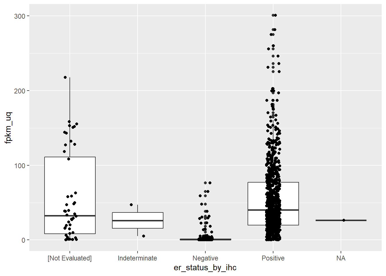

Phew! So ESR1 expression is indeed higher in ER positive samples. The plot also highlights some discrepancy in the recording of the ER status which should be cleaned prior to analysis. For the sake of the plot we can filter out the offending entries.

brca_fpkm_uq_unstrand[rowData(brca_fpkm_uq_unstrand)$gene_name == "ESR1"] %>% 
  tidybulk() %>% 
  filter(er_status_by_ihc %in% c("Positive", "Negative")) %>% 
  ggplot(aes(x = er_status_by_ihc, y = fpkm_uq)) + geom_boxplot() + geom_jitter(width = 0.1) + xlab("ER Status")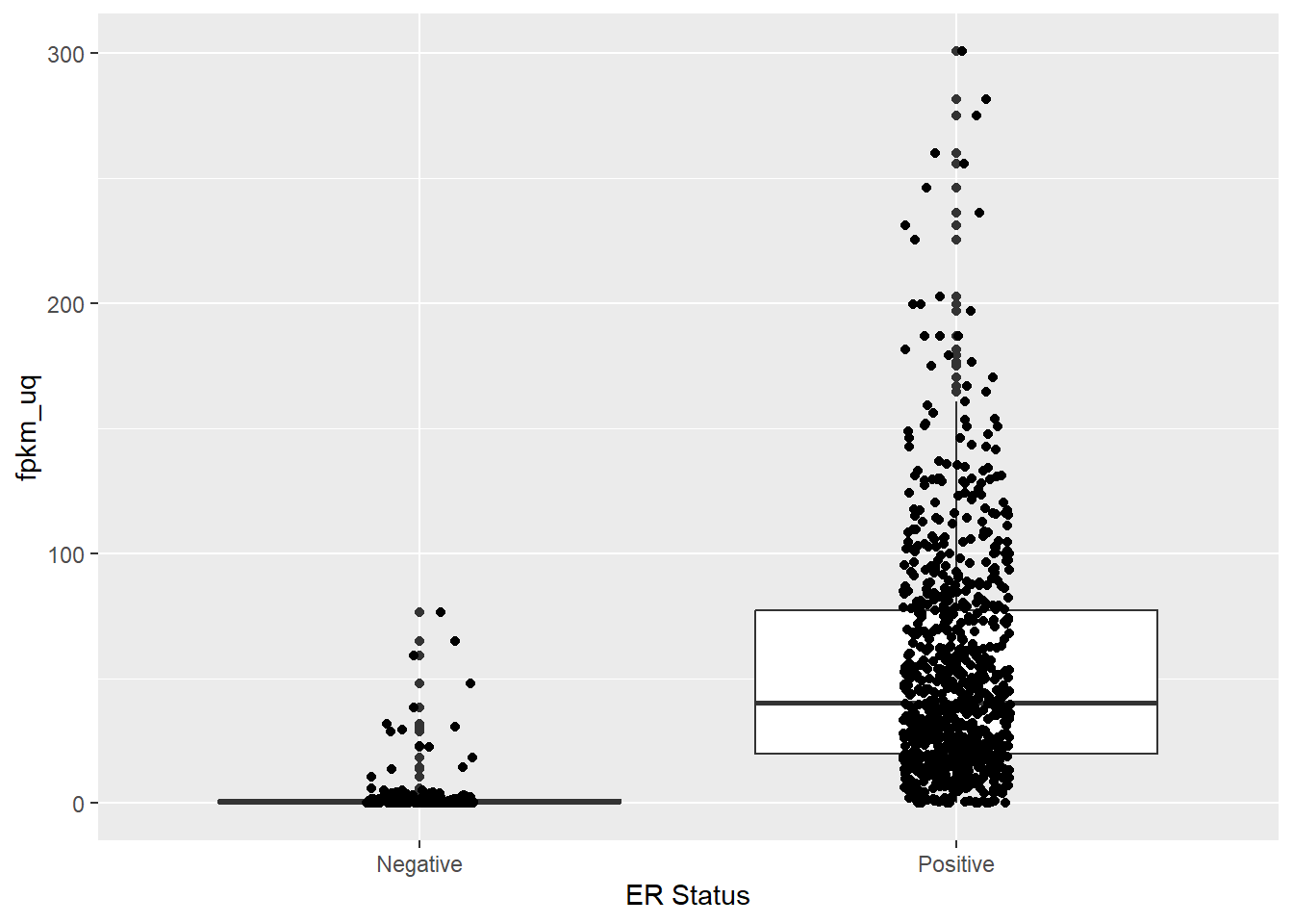

In a similar vein, the gene ERBB2 should be higher in patients that are positive for Her2 staining by IHC.

brca_fpkm_uq_unstrand[rowData(brca_fpkm_uq_unstrand)$gene_name == "ERBB2"] %>% 
  tidybulk() %>% 
  filter(her2_status_by_ihc %in% c("Positive", "Negative")) %>% 
  ggplot(aes(x = her2_status_by_ihc, y = fpkm_uq)) + geom_boxplot() + geom_jitter() + scale_y_log10()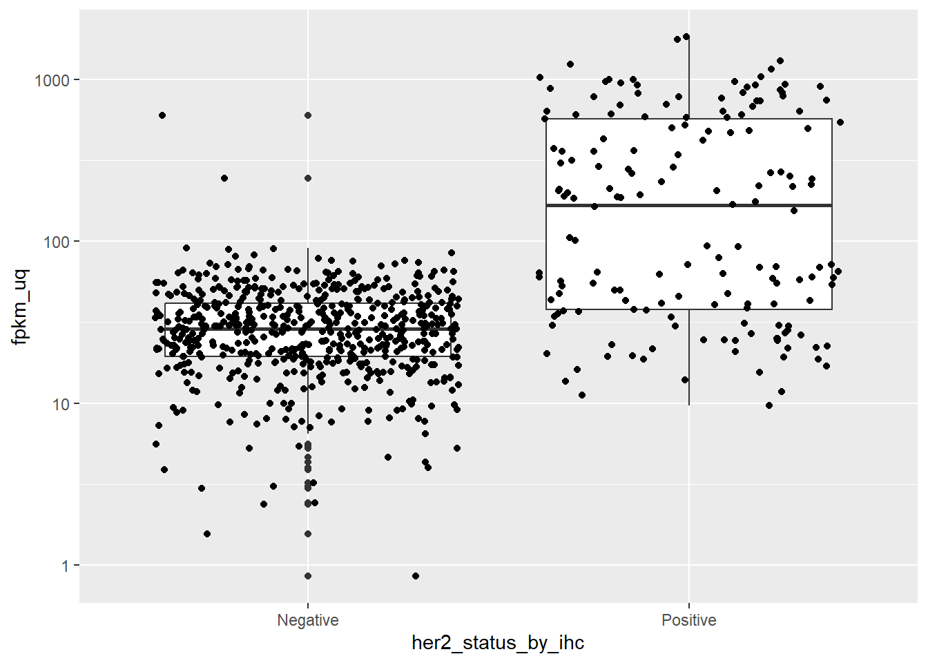

Breast cancer was traditionally classified into five intrinsic subtypes, and microarray studies sought to identify genes that define these subtypes. On such 50 gene panel was derived using a prediction analysis of microarray (PAM) and hence called PAM50. The samples in the TCGA dataset have been classified using this method, and we can check the expression level of ESR1 and ERBB2 respectively.

brca_fpkm_uq_unstrand[rowData(brca_fpkm_uq_unstrand)$gene_name %in% c("ESR1","ERBB2")] %>% 
  tidybulk() %>% 
  filter(!is.na(paper_BRCA_Subtype_PAM50)) %>% 
  ggplot(aes(x = paper_BRCA_Subtype_PAM50, y = fpkm_uq, fill = paper_BRCA_Subtype_PAM50)) + 
  geom_boxplot() + 
  geom_jitter(alpha=0.1) + 
  scale_y_log10() + 
  facet_wrap(~gene_name) + 
  scale_fill_manual(values = c("red", "pink", "darkblue", "lightblue", "yellow"))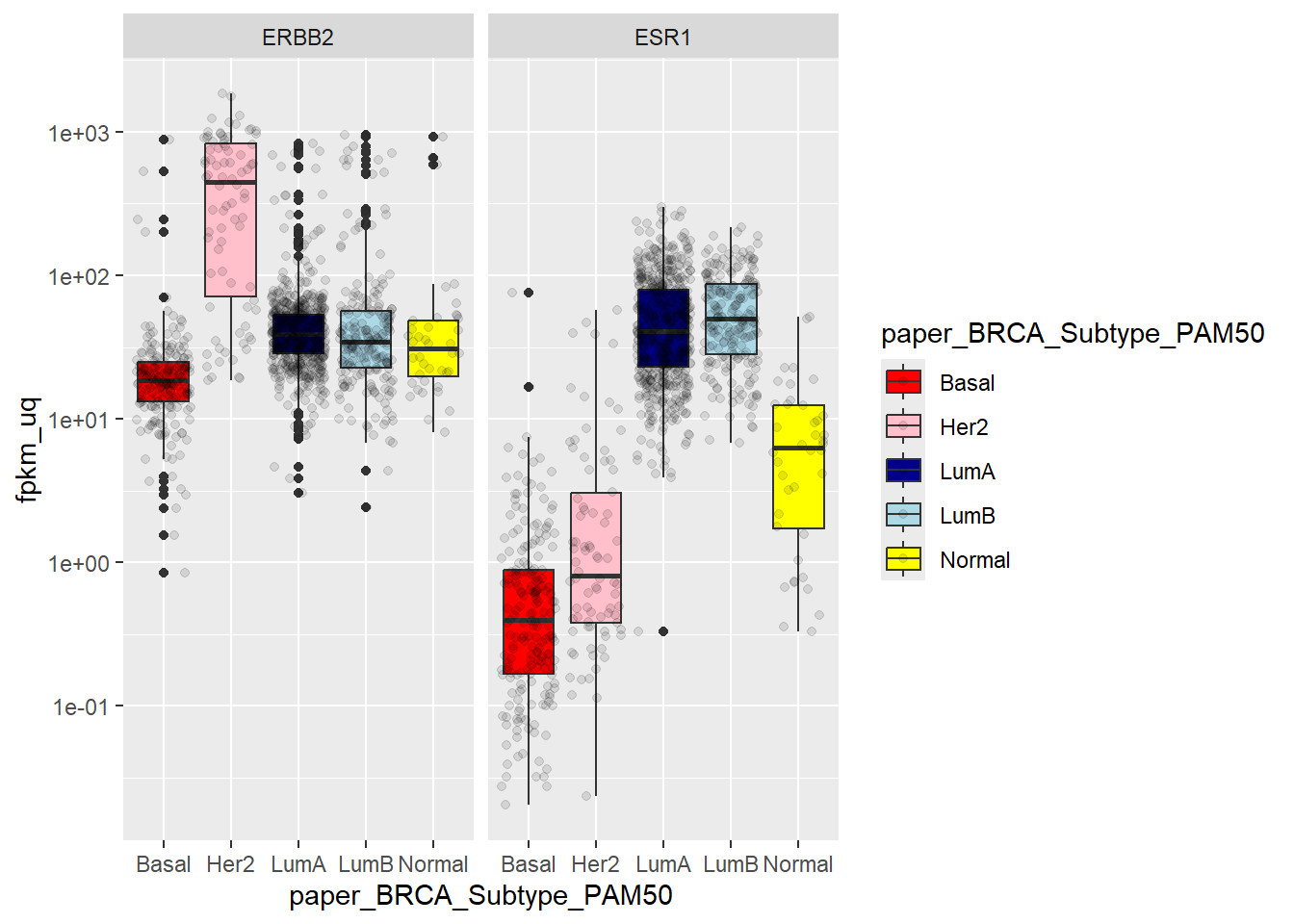

Again, this all makes perfect sense as Luminal A and Luminal B are ER-positive groups, Basal and Her2 are ER-negative and ERBB2 should be highly expressed in the Her2 subtype.

So, are the Pam50 subtypes are major source of variation in our data? The tidybulk package allows us to run dimensionality reduction techniques such as PCA to look at this issue. The reduce_dimensions function computes the Principal Components and these can be added to our data ready for visualisation. Normally tidybulk would require a scale_abundance step here to correct for differences in sequencing depth between samples, but since we are using values that are already normalised to some extent this is not needed on this ocassion.

brca_fpkm_uq_unstrand |>
  reduce_dimensions(method = "PCA")  |> 
  ## not needed here: scale_abundance() |>
  pivot_sample()  |>
  select(.sample, PC1, PC2)

# A tibble: 1,111 × 3
   .sample                         PC1    PC2
   <chr>                         <dbl>  <dbl>
 1 TCGA-EW-A2FS-01A-11R-A17B-07  9.35  -8.84 
 2 TCGA-OL-A6VR-01A-32R-A33J-07 -6.26  -4.46 
 3 TCGA-E9-A226-01A-21R-A157-07 -8.62   4.47 
 4 TCGA-A8-A08H-01A-21R-A00Z-07  0.362  5.87 
 5 TCGA-D8-A27H-01A-11R-A16F-07  7.76  16.8  
 6 TCGA-D8-A3Z6-01A-11R-A239-07 -5.76  -5.94 
 7 TCGA-B6-A1KN-01A-11R-A13Q-07  0.728  0.144
 8 TCGA-BH-A0DL-01A-11R-A115-07 20.8    6.48 
 9 TCGA-A8-A09X-01A-11R-A00Z-07 13.6   -4.60 
10 TCGA-BH-A2L8-01A-11R-A18M-07  5.41  -7.91 
# ℹ 1,101 more rows

It is now straightforward to plot, and also colour according to the PAM50 subtype of each sample.

brca_fpkm_uq_unstrand |> 
  reduce_dimensions(method = "PCA")  |>
  pivot_sample()  |>
  filter(!is.na(paper_BRCA_Subtype_PAM50))  |>
  ggplot(aes(x = PC1, y = PC2, col = paper_BRCA_Subtype_PAM50 )) + 
  geom_point()  + 
  scale_color_manual(values = c("red", "pink", "darkblue", "lightblue", "yellow"))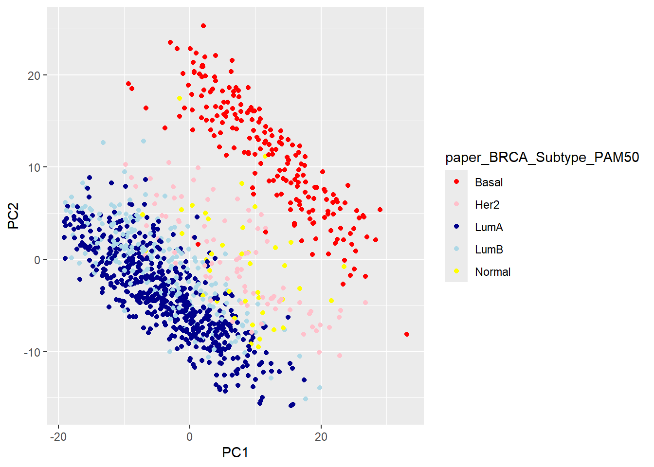

A heatmap of genes from the literature

The PCA looks pretty good, with the main separation being between basal and Luminal A/B. Furthermore, we can get from the literature the names of the genes used in the PAM50 classifier. I got these from the genefu Bioconductor package and saved as a small text file. My previous go-to package for heatmaps was pheatmap, but whilst writing this up I came across tidyHeatmap

tidyHeatmap

This package works quite well with our workflow of using a “tidy” framework. It requires data in a tbl_df or tibble format, which we can create from tidybulk once we are done with pre-processing the data. Although the data we are working with are normalised, we must apply a log\(_2\) transformation for the purposes of visualisation. I’ve also applied some basic data cleaning

The tidyHeatmap function heatmap allows us to quickly add sample annotations to the plot, and since our data were using the tidy framework we have plenty of clinical variables at our fingertips. I’m choosing ER status and PAM50 classification, but you could add others such age, grade, or anything else.

if(!file.exists("PAM50_genes.txt")) download.file("https://raw.githubusercontent.com/markdunning/markdunning.github.com/refs/heads/master/posts/2025_11_06_tidymodels_TCGA_part1/PAM50_genes.txt", destfile = "PAM50_genes.txt")

pam50_genes <- read.table("PAM50_genes.txt")[,1]

library(tidyHeatmap)

 brca_fpkm_uq_unstrand[rowData(brca_fpkm_uq_unstrand)$gene_name %in% pam50_genes,] %>% 
  ## once filtered, make a "tidy" version
  tidybulk() %>% 
  mutate(logcount = log2(fpkm_uq + 1)) %>% 
  ## get the counts, samples and genes
  rename(ER = er_status_by_ihc, PAM50 =paper_BRCA_Subtype_PAM50) %>%
  as_tibble() %>% 
  mutate(ER = ifelse(ER %in% c("Positive", "Negative"), ER, NA)) %>% 
  filter(!is.na(ER), !is.na(PAM50)) %>% 
  tidyHeatmap::heatmap(
        .column = .sample,
        .row = gene_name,
        .value = logcount,   
        scale = "row",
        palette_value = circlize::colorRamp2(
            seq(-5, 5, length.out = 11), 
            RColorBrewer::brewer.pal(11, "RdBu")
        )
    ) %>% 
  annotation_tile(ER ,palette = c("orange","purple")) %>% 
  ## I couldn't work out how to assign particular colours, so had to experiment at bit with the correct order to specify the colours in
  annotation_tile(PAM50,palette = c("darkblue", "pink", "lightblue", "yellow", "red"))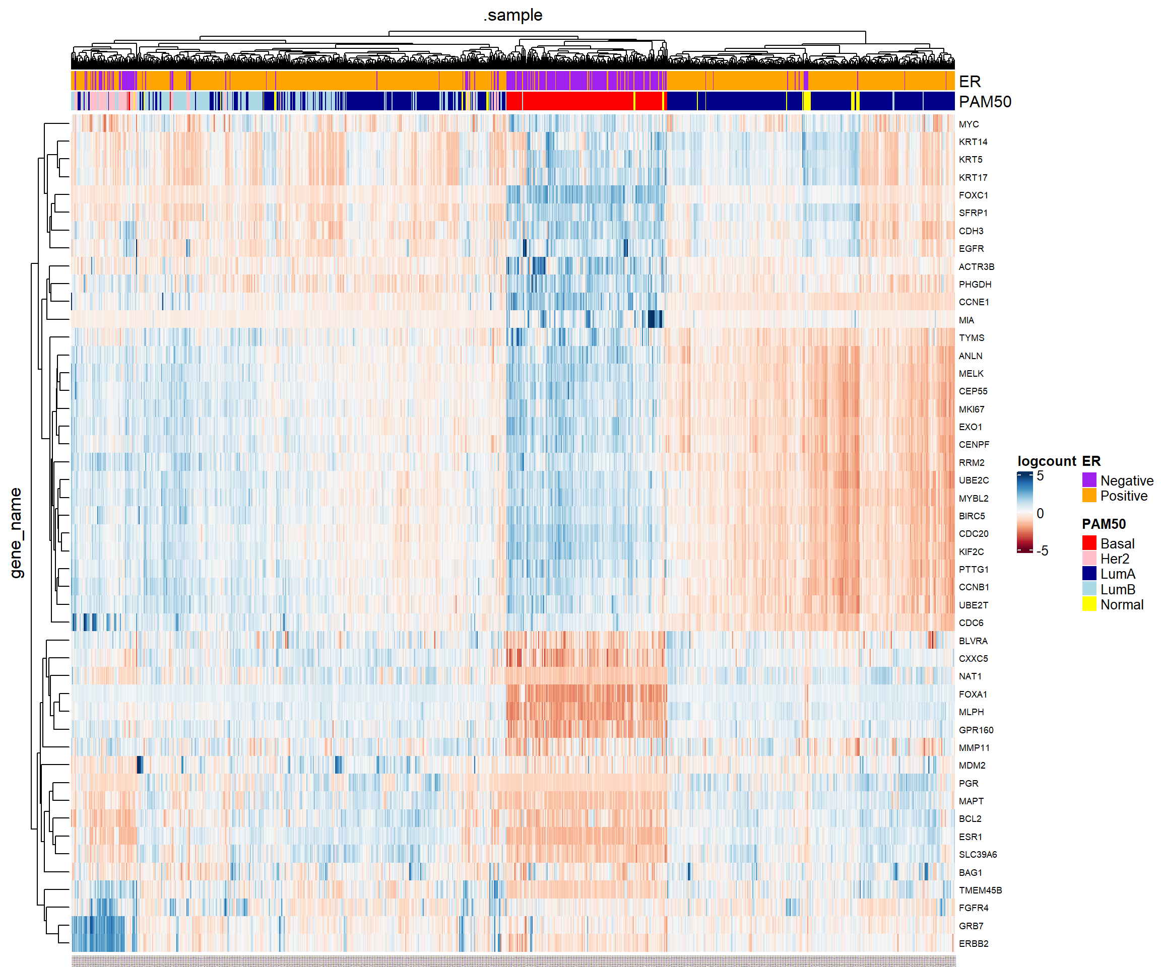

Showing the data in this manner also us to see which genes look to be over- or under-expressed in certain subtypes. Eventually, we will progress to doing our own classification so it will be useful to compare to this information.

Survival Analysis

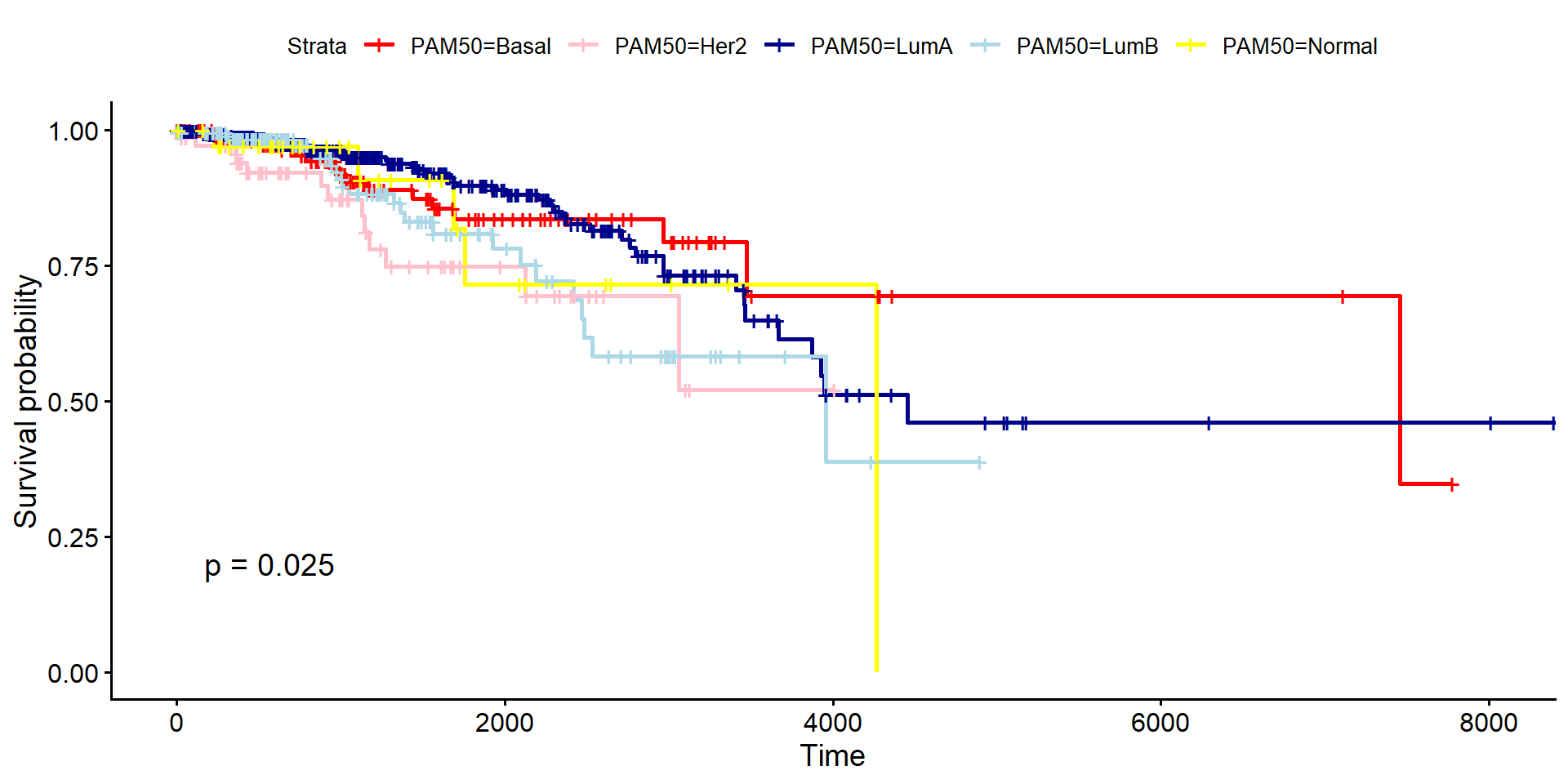
Finally, a pertinent question to ask is whether the subtypes are clinically-meaningful. If we know what subtype a patient has, what can this tell us about their survival prospects? A kaplan-meier (KM) curve is a standard way to estimate and visualize the survival probability over a specified period, and can be created by the survival package and visualised using the package survminer. The curve starts at 100% (or probability 1.0) at time zero and steps down each time a patient dies. A tick mark on the curve indicates a patient who was lost to follow-up or was still alive when the data was collected (censored). These patients contribute to the probability calculation up until the time they were last observed.

The clinical data we have needs modifying slightly to run the analysis. In particular we need to create “Status” and “Time” columns which records if a patient is alive (0) or dead (1) at the end of the study, and the time to either death or total follow-up time. We will also remove any patients where the Time or status is missing or inaccurate. The dataset also includes some metastatic or recurrent tumours, but for the purposes of the curve we will use only “primary” samples.

library(survminer)
library(survival)
clin_data_corrected <- colData(brca_fpkm_uq_unstrand) %>% 
  data.frame() %>% 
  dplyr::filter(classification_of_tumor == "primary") %>% 
  #Define Time (Coalesce death date and follow-up date)
  dplyr::mutate(
    # Use days_to_death if available; otherwise, use days_to_last_follow_up
    Time = as.numeric(dplyr::coalesce(days_to_death, days_to_last_follow_up)),
    # Define Status 
    # Event=1 (Dead), Censored=0 (Alive)
    Status = ifelse(vital_status.x == "Dead", 1, 0)
  ) |>
  # Remove rows with NA in Time, Status, or Subtype
  dplyr::filter(!is.na(Time), Time > 0, Status %in% c(0, 1), paper_BRCA_Subtype_PAM50 != "NA") |>
  dplyr::mutate(PAM50 = paper_BRCA_Subtype_PAM50)

Running the analysis and plotting can then be achieved using the survfit and ggsurvplot packages respectively. The p-value requested is the p-value for there being any difference in survival between different groups and is calculated using a log-rank test.

# --- Run Survival Analysis ---
fit <- survfit(Surv(Time, Status) ~ PAM50, data = clin_data_corrected)

# --- Plot ---
ggsurvplot(
  fit, 
  data = clin_data_corrected, 
  pval = TRUE,
  palette = c("red", "pink", "darkblue", "lightblue", "yellow")
)

There are plenty more examples on the survminer website on how to customise this further

Preparing the data for Machine Learning

The machine learning tasks we have planned require a slightly different strategy for processing. Firstly, whist FPKM are an easy way to compare expression across different gene lengths and library sizes for visualization, it’s not a statistically robust input for advanced modeling tasks. For the most reliable and highest-performing model(s), particularly when using linear methods the input data must adhere to statistical assumptions (such as a stable variance across the whole range of counts). Furthermore, FPKM incorporates cohort-level information during calibration. A central tenent of Machine Learning is that data are dividing into training and testing sets that crucially are processed completely independently such that no information from the testing set is used during training. The cohort-level nature of FPKM violates this assumption and potentially leads to an issue called “data leakage” which could compromise the validity of our models and lead to overly-optimistic predictions.

We will therefore take the raw counts from TCGA as our stating point. Our approach will be to first split the data into independent training and testing sets, and then process the training data. Our testing data will be transformed using parameters learnt from the training data. Finally, we will state our intentions of modeling the Estrogen Receptor (ER) status and therefore include only samples where we have a Positive or Negative observations for this variable.

First we will create a matrix of raw counts of all available samples.

library(tidymodels)
library(DESeq2)

set.seed(42)

## Load the full dataset we created previously

brca.data_full <- readRDS("brca.data_full.rds")

tcga_brca.clin <- readr::read_tsv("tcga_brca.clin.tsv", show_col_types = FALSE)

# get the gene annotations stored in the full data
gene_info <- rowData(brca.data_full)

## Join the sample information extra clinical variables
## Add the barcode as rownames, which will make subsetting easier

sample_info <- colData(brca.data_full) |>
  data.frame() |>
  dplyr::left_join(tcga_brca.clin, by = c("patient"="bcr_patient_barcode")) %>% 
  filter(er_status_by_ihc %in% c("Positive","Negative")) %>% 
  tibble::column_to_rownames("barcode")

raw_assay <- assay(brca.data_full, "unstranded")[,rownames(sample_info)] 
rownames(raw_assay) <- gene_info$gene_name

It is possible to use the sample function from R to pick rows from our dataset, or even the slice_sample from dplyr, but the most straightforward way of splitting the data into training and testing is using the tidymodels package. We will learn lots about this package in due course. The same way that tidyverse is a collection of packages with a common philosophy for data manipulation and visualisaton, tidymodels is a ecosystem of packages for all steps of machine learning. The first task is often to split data into training and testing sets, which is performed by the initial_split function after loading tidymodels. During the split it is common to use the majority (say 80%) of the data for training. You can also make sure that the your outcome of interest has roughly the same proportion in training and testing.

Once a split is created with initial_split you can extract the training and testing data. We actually just want the barcodes of the training and testing sets, and we can use these to create DESeq2 objects from the raw counts.

library(tidymodels)
library(DESeq2)

set.seed(42)

data_split <- data.frame(Sample = rownames(sample_info), ER = sample_info$er_status_by_ihc) %>% 
  initial_split(prop = 0.8, strata  = "ER")

training_samples <- training(data_split) %>% pull(Sample)
testing_samples <- testing(data_split) %>% pull(Sample)

brca_training <- DESeqDataSetFromMatrix(raw_assay[,training_samples],
                                        sample_info[training_samples,],
                                        design = ~er_status_by_ihc)

brca_testing <- DESeqDataSetFromMatrix(raw_assay[,testing_samples],
                                        sample_info[testing_samples,],
                                        design = ~er_status_by_ihc)

We now perform the statistical normalization, variance stabilization, and feature selection steps, ensuring that all parameters are calculated solely from the training data before being applied consistently to both sets.

The DESeq2 function estimateSizeFactors() calculates a normalization factor for each sample (a column) in the training set. This accounts for differences in sequencing depth (library size). This must be calculated first, as it is needed for the subsequent steps. The estimateDispersions() function then calculates the gene-wise biological variability. Critically, it fits a function that models the relationship between a gene’s mean expression and its variance across the entire training cohort. Once estimated, this function can be added directly to the testing data to ensure both training and testing data are processed the same.

We convert the normalized counts to a log\(_2\) scale (adding the essential \(+1\) pseudo-count to handle zeros). This transformation helps stabilize the variance but, more importantly here, makes the variance calculation reflective of biological fold change rather than raw magnitude. We choose the Top 250 Most Variable Genes for two reasons to combat the “Curse of Dimensionality” by reducing the feature space. This step calculates the variability only on the training data, preventing “leakage”. The resulting list, most_var_genes, is the filter to be used for both sets.

estimateSizeFactors() is run independently on the test data, which is fine because size factors are a sample-specific property (based on that sample’s own depth) and do not leak cohort information.

brca_training <- estimateSizeFactors(brca_training)
brca_training <- estimateDispersions(brca_training)

normalised_counts <- log2(counts(brca_training, normalized = TRUE) + 1)

most_var_genes <- rownames(normalised_counts)[order(rowVars(normalised_counts),decreasing = TRUE)[1:250]]

brca_testing <- estimateSizeFactors(brca_testing)
dispersionFunction(brca_testing) <- dispersionFunction(brca_training)

Finally we perform the VST step to calibrate both datasets, and then convert to a “tidy” format that we will need for machine learning.

vsd_train <- varianceStabilizingTransformation(brca_training, blind = FALSE)
vsd_test <- varianceStabilizingTransformation(brca_testing, blind = FALSE)

brca_train_tidy <- assay(vsd_train)[most_var_genes,] %>% 
  t() %>% 
  data.frame() %>% 
  tibble::rownames_to_column("barcode") %>% 
  left_join(tibble::rownames_to_column(sample_info, "barcode"))

brca_test_tidy <- assay(vsd_test)[most_var_genes,] %>% 
  t() %>% 
  data.frame() %>% 
  tibble::rownames_to_column("barcode") %>% 
  left_join(tibble::rownames_to_column(sample_info, "barcode"))

saveRDS(brca_train_tidy, "brca_train_tidy.rds")
saveRDS(brca_test_tidy, "brca_test_tidy.rds")

Next time

Make sure the tidy filtered objects brca_train_tidy.rds and brca_test_tidy.rds are saved for next time and we will start some machine learning tasks.