Introduction to RNA-Seq - Part 2

Performing differential expression on Bulk RNA-seq data using DESeq2

Author

Mark Dunning

Published

October 25, 2025

Quick Start

This section follows on from Part 1 where we saw how to import raw RNA-seq counts into DESeq2 and perform some quality assessment. Several packages are required, which can be downloaded with this code:-

source("https://raw.githubusercontent.com/markdunning/markdunning.github.com/refs/heads/master/files/training/bulk_rnaseq/install_bioc_packages.R")

The following will also assume you have created a DESeq2 object in a folder called Robjects in your working directory. This can be downloaded with the following.

dir.create("Robjects/",showWarnings = FALSE)
download.file("https://github.com/markdunning/markdunning.github.com/raw/refs/heads/master/files/training/bulk_rnaseq/dds.rds",destfile = "Robjects/dds.rds")

Differential expression with `DESeq2`

Now that we are happy that the data quality looks good, we can proceed to test for differentially expressed genes. There are a number of packages to analyse RNA-Seq data. Most people use DESeq2, edgeR or limma. We will use DESeq2 for the rest of this practical.

Recap of pre-processing

The previous section walked-through the pre-processing and transformation of the count data. Here, for completeness, we list the minimal steps required to process the data prior to differential expression analysis.

Note that although we spent some time looking at the quality of our data , these steps are not strictly necessary prior to performing differential expression so are not shown here for the sake of brevity. Remember, DESeq2 requires raw counts so the vst transformation is not shown as part of this basic protocol.

library(DESeq2)

count_file <- "raw_counts/raw_counts_matrix.tsv"
counts <- read.delim(count_file)

## Step needed for this data to tidy the column names
colnames(counts)[-1] <- stringr::str_remove_all(colnames(counts)[-1], "X")

sampleinfo_corrected <- read.delim("meta_data/sampleInfo_corrected.txt")
dds <- DESeqDataSetFromMatrix(counts, 
                                colData = sampleinfo_corrected,
                                design = ~condition, tidy=TRUE)

saveRDS(dds, file="Robjects/dds.rds")

We will be using these raw counts throughout the workshop and transforming them using methods in the DESeq2 package. If you want to know about alternative methods for count normalisation they are covered on this page.

The DESeq workflow in brief

We have previously defined the condition as our factor of interest using the design argument when we created the object. This can be checked using the design function. The current design can be queried using the design function.

design(dds)

~condition

It can be changed at any point before we run the differential expression workflow, can refer to any of the variables saved in the colData of the dds object, or even a combination of different variables.

colData(dds)

DataFrame with 9 rows and 5 columns
                    Run condition        Name Replicate     Treated
            <character>  <factor> <character> <integer> <character>
1_CTR_BC_2   1_CTR_BC_2       CTR       CTR_1         1           N
2_TGF_BC_4   2_TGF_BC_4       TGF       TGF_1         1           Y
3_IR_BC_5     3_IR_BC_5       IR         IR_1         1           Y
4_CTR_BC_6   4_CTR_BC_6       CTR       CTR_2         2           N
5_TGF_BC_7   5_TGF_BC_7       TGF       TGF_2         2           Y
6_IR_BC_12   6_IR_BC_12       IR         IR_2         2           Y
7_CTR_BC_13 7_CTR_BC_13       CTR       CTR_3         3           N
8_TGF_BC_14 8_TGF_BC_14       TGF       TGF_3         3           Y
9_IR_BC_15   9_IR_BC_15       IR         IR_3         3           Y

The counts that we have obtained via sequencing are subject to random sources of variation. The purpose of differential expression is to determine if potential sources of biological variation (e.g. counts observed from different sample groups) are greater than random noise.

The DESeq function is the main workflow for differential expression and runs a couple of processing steps automatically to adjust for different library size and gene-wise variability. You can you can read about these in the DESeq2 vignette and run some example code at the end of this session.

de_condition <- DESeq(dds)

estimating size factors

estimating dispersions

gene-wise dispersion estimates

mean-dispersion relationship

final dispersion estimates

fitting model and testing

de_condition

class: DESeqDataSet 
dim: 57914 9 
metadata(1): version
assays(4): counts mu H cooks
rownames(57914): ENSG00000000003 ENSG00000000005 ... ENSG00000284747
  ENSG00000284748
rowData names(26): baseMean baseVar ... deviance maxCooks
colnames(9): 1_CTR_BC_2 2_TGF_BC_4 ... 8_TGF_BC_14 9_IR_BC_15
colData names(6): Run condition ... Treated sizeFactor

The results of the analysis are not immediately accessible, but can be obtained using the results function.

results(de_condition)

log2 fold change (MLE): condition TGF vs CTR 
Wald test p-value: condition TGF vs CTR 
DataFrame with 57914 rows and 6 columns
                   baseMean log2FoldChange     lfcSE       stat     pvalue
                  <numeric>      <numeric> <numeric>  <numeric>  <numeric>
ENSG00000000003 1430.562846     -0.2562067 0.0813936 -3.1477521 0.00164531
ENSG00000000005    0.113566     -0.0883933 4.0804559 -0.0216626 0.98271709
ENSG00000000419 1790.537536     -0.1449058 0.1008195 -1.4372794 0.15063862
ENSG00000000457  640.692302     -0.3106360 0.1137555 -2.7307347 0.00631933
ENSG00000000460  206.179026      0.1600274 0.1567963  1.0206074 0.30744046
...                     ...            ...       ...        ...        ...
ENSG00000284744    8.307038      -0.209531  0.800702  -0.261684   0.793565
ENSG00000284745    0.000000             NA        NA         NA         NA
ENSG00000284746    0.101097      -1.050150  4.080456  -0.257361   0.796900
ENSG00000284747   28.783710      -0.297530  0.448931  -0.662751   0.507490
ENSG00000284748    0.548323       0.873372  4.080456   0.214038   0.830517
                      padj
                 <numeric>
ENSG00000000003 0.00906995
ENSG00000000005         NA
ENSG00000000419 0.30807839
ENSG00000000457 0.02685529
ENSG00000000460 0.50350287
...                    ...
ENSG00000284744         NA
ENSG00000284745         NA
ENSG00000284746         NA
ENSG00000284747   0.689074
ENSG00000284748         NA

Each row is a particular gene measured in the study (i.e. all genes in the organism being studied) and each column reports some aspect of the differential expression analysis for that gene. The values that I typically pay most attention to are highlighted in bold.

Column Name	Description	Importance
baseMean	The average of normalized count values (size-factor corrected) across all samples in the comparison.	Measures the average expression magnitude of the gene and useful for basic filtering
log2FoldChange	The estimated log base 2 fold change between the two groups being contrasted (e.g., Treatment / Control).	The primary measure of the effect size or magnitude of the difference.
lfcSE	The standard error estimate for the \(\text{log}_2\text{FoldChange}\).	Measures the precision of the \(\text{log}_2\text{FC}\) estimate. Smaller values indicate higher reliability.
stat	The Wald test statistic (calculated as \(\text{log}_2\text{FC} / \text{lfcSE}\))	The statistical value used to test the null hypothesis (that the \(\text{log}_2\text{FC}\) is zero)
pvalue	The \(p\)-value derived from the Wald test statistic.	The unadjusted probability of observing the effect by chance. Do not use this for filtering.
padj	The Benjamini-Hochberg adjusted \(p\)-value (False Discovery Rate, FDR).CRITICAL for significance. This corrects for multiple testing	CRITICAL for statistical significance. This corrects for multiple testing. Genes are considered differentially expressed if this value is below your threshold (e.g., 0.05).

Note that all genes are reported. At this stage the gene identifiers are not very informative, something we will fix shortly. Furthermore, the results function displays results in a format which is not compatible with standard data manipulation tools (i.e. tidyverse), so we will have to convert.

Processing the DE results using tidyverse

The output can be converted into a data frame and manipulated in the usual manner if we add the tidy = TRUE argument to results. It is recommended to use dplyr to manipulate the data frames with the standard set of operations detailed on the dplyr cheatsheet

select to pick which columns to display
filter to restrict the rows
mutate to add new variables to the data frame
arrange to order the data frame according to values of a column or columns

A tidy framework for RNA-seq

There is actually a dedicated workflow for those familiar with “tidy” methodologies and wish to apply the same philosophy to RNA-seq and other ’omics data. I plan to cover this at a later point.

the tidybulk page

Neither the tidybulk or approach I present here is necessarily better than the other, and should in fact yield exactly the same results.

library(dplyr)
 results(de_condition, tidy=TRUE) %>% 
   slice_head(n=10)

               row     baseMean log2FoldChange      lfcSE       stat
1  ENSG00000000003 1430.5628457    -0.25620674 0.08139356 -3.1477521
2  ENSG00000000005    0.1135661    -0.08839330 4.08045587 -0.0216626
3  ENSG00000000419 1790.5375358    -0.14490579 0.10081950 -1.4372794
4  ENSG00000000457  640.6923020    -0.31063596 0.11375545 -2.7307347
5  ENSG00000000460  206.1790264     0.16002744 0.15679627  1.0206074
6  ENSG00000000938    7.4126750    -1.94966011 0.94841767 -2.0556978
7  ENSG00000000971 5318.4200170    -0.37348479 0.06859390 -5.4448693
8  ENSG00000001036 3629.7262081    -0.42700955 0.05618654 -7.5998545
9  ENSG00000001084  923.1202025    -0.19549932 0.09925106 -1.9697455
10 ENSG00000001167 1261.1547094     0.08263564 0.09065646  0.9115251
         pvalue         padj
1  1.645312e-03 9.069945e-03
2  9.827171e-01           NA
3  1.506386e-01 3.080784e-01
4  6.319333e-03 2.685529e-02
5  3.074405e-01 5.035029e-01
6  3.981166e-02           NA
7  5.184345e-08 9.308987e-07
8  2.964639e-14 1.176542e-12
9  4.886755e-02 1.346109e-01
10 3.620188e-01 5.605916e-01

Note

Although, the “tidy” output is more useful for downstream analysis, I personally like the output generated by the results function without tidy=TRUE as it displays the contrast being tested (in this case TGF vs CTR). This is a good way of checking that you are comparing the groups that you expect.

We can sort the rows by adjusted p-value and then print the first 10 rows. I’m using slice_head function as a dplyr equivalent to the base head.

results(de_condition,tidy=TRUE) %>%
  arrange(padj) %>%  
  slice_head(n=10)

               row    baseMean log2FoldChange      lfcSE     stat        pvalue
1  ENSG00000119681   6471.7058       2.372065 0.07076496 33.52033 2.437260e-246
2  ENSG00000120708  22001.6982       1.436637 0.05904590 24.33084 9.248277e-131
3  ENSG00000172061   1481.6147       2.384971 0.09843523 24.22883 1.105455e-129
4  ENSG00000049540    932.0366       3.999465 0.17556867 22.78006 7.228861e-115
5  ENSG00000060718   1512.0092       2.123432 0.09532775 22.27506 6.448803e-110
6  ENSG00000115414 683348.5240       1.453310 0.06867840 21.16109  2.181368e-99
7  ENSG00000187498  30609.2525       1.458950 0.06926943 21.06196  1.776880e-98
8  ENSG00000186340  14380.2024       1.468632 0.06999698 20.98136  9.707600e-98
9  ENSG00000087245  51862.2917       1.282562 0.06613894 19.39194  9.026914e-84
10 ENSG00000139211   2302.3470       2.070441 0.10902113 18.99119  2.017183e-80
            padj
1  4.371957e-242
2  8.294780e-127
3  6.609883e-126
4  3.241783e-111
5  2.313573e-106
6   6.521564e-96
7   4.553383e-95
8   2.176687e-94
9   1.799164e-80
10  3.618422e-77

Or we can sort the rows and then write the resulting data frame to a file.

File naming

You can name the csv as anything - although something like results.csv is probably not particularly helpful for all but the simplest datasets. Personally, I like to choose file names that are informative about the contents even if they do look a bit complicated.

dir.create("de_analysis",showWarnings = FALSE)
 results(de_condition,tidy=TRUE) %>%
  arrange(padj) %>% 
   readr::write_csv("de_analysis/condition_TGF_vs_CTR_DESeq_all.csv")

Filtering to the differentially-expressed genes can be achieved using the filter function from dplyr with some cut-off on the adjusted p-value.

 results(de_condition,tidy=TRUE) %>%
  filter(padj < 0.05) %>% 
  readr::write_csv("de_analysis/condition_TGF_vs_CTR_DESeq_sig.csv")

It is also a good idea to save the DESeq output object itself so we can re-use later.

saveRDS(de_condition, file="Robjects/de_condition.rds")

We can discover how many differentially-expressed genes (at a particular p-value cut-off) using the count function. I am making sure that I explicitly use the count function from dplyr using the technique of putting dplyr:: before count.

results(de_condition,tidy=TRUE) %>%
  dplyr::count(padj < 0.05)

  padj < 0.05     n
1       FALSE 13039
2        TRUE  4899
3          NA 39976

Note

You may notice the amount of NA p-values here. We will come back to this later, but it is related to some filtering that DESeq2 is doing as default.

Another overview of the results is to use the plotMA function. Each point on this plot represents and individual gene with the x- and y-axes being the overall expression level and magnitude of difference respectively. Statistically significant genes are automatically highlighted. The fanning effect at low expression levels is often seen due to high relative fold-change at low expression levels. Once you have run your DE analysis, an MA plot visually confirms that your DE genes are not exclusively confined to extremely low-count regions.

plotMA(de_condition)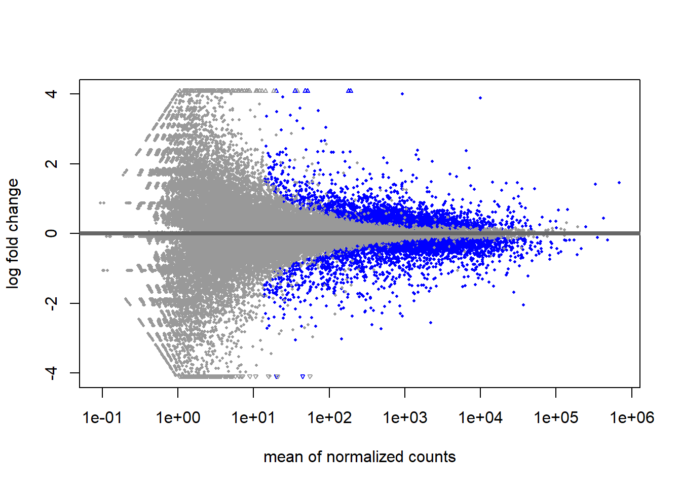

It is also instructive to perform a “sanity” check and plot the sample-level counts for genes with high significance. This could highlight any other technical factors that we are not currently taking into account. The plot is not particularly attractive, but is a good quick diagnostic as it confirms which direction your contrast is. i.e. Treatment vs Control or Control vs Treatment.

## Get the gene lowest p-value and a log2 fold-change over 0

top_up <- results(de_condition, tidy = TRUE) %>% 
  filter(log2FoldChange > 0) %>% 
  slice_min(padj) %>% 
  pull(row)
plotCounts(dds,top_up,intgroup = "condition")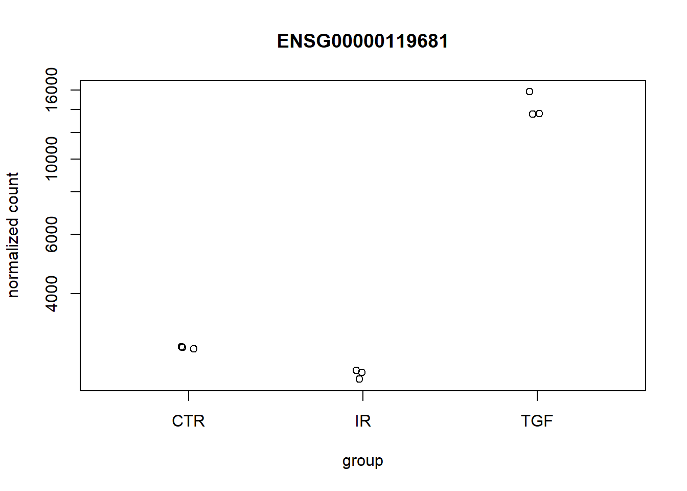

## Get the gene with the lowest p-value and a log2 fold-change less than 0
top_down <- results(de_condition, tidy = TRUE) %>% 
  filter(log2FoldChange < 0) %>% 
  slice_min(padj) %>% 
  pull(row)

plotCounts(dds,top_down,intgroup = "condition")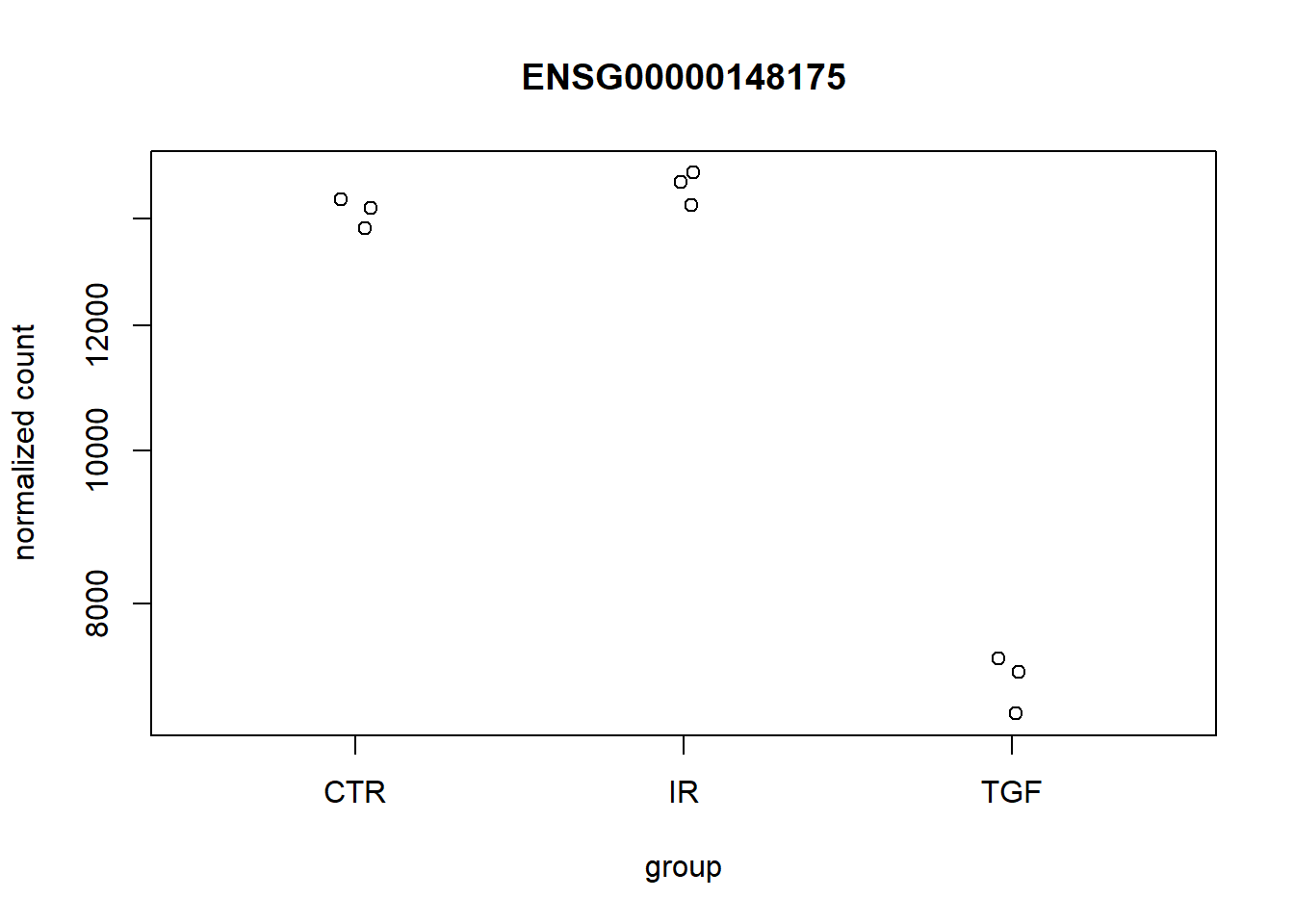

Note

If your study involves knocking-out a particular gene, or you have some positive controls that are known in advance, it would be a good idea to visualise their expression level with plotCounts.

Changing the direction of the contrast, or the groups being compared

You hopefully noticed that the sign of the log fold changes have been calculated using the CTR group as a baseline. In other words, a positive log2FoldChange means that a gene has higher expression in TGF compared to CTR. This is usually the direction that makes sense for biological interpretation. However, DESeq2 has not done anything clever here. The order of the contrasts is dictated by the “levels” of the variable used in the design.

dds$condition

[1] CTR TGF IR  CTR TGF IR  CTR TGF IR 
Levels: CTR IR TGF

Since CTR is the first thing printed here it gets chosen as the baseline. It is just a fortunate coincidence that CTR is first alphabetically! In order that we are not relying on the defaults and for transparency, I tend to explicitly state which contrast I want to make using the contrast argument and have full control over what the baseline is. In the contrast argument you create a vector (using c) followed by the levels in the order you want to compare with the baseline coming last.

In the below this can be read as TGF vs CTR, which is in fact the default

## This should give the same as the table above
results(de_condition, contrast=c("condition","TGF","CTR"))

log2 fold change (MLE): condition TGF vs CTR 
Wald test p-value: condition TGF vs CTR 
DataFrame with 57914 rows and 6 columns
                   baseMean log2FoldChange     lfcSE      stat     pvalue
                  <numeric>      <numeric> <numeric> <numeric>  <numeric>
ENSG00000000003 1430.562846      -0.256207 0.0813936  -3.14775 0.00164531
ENSG00000000005    0.113566       0.000000 4.0804559   0.00000 1.00000000
ENSG00000000419 1790.537536      -0.144906 0.1008195  -1.43728 0.15063862
ENSG00000000457  640.692302      -0.310636 0.1137555  -2.73073 0.00631933
ENSG00000000460  206.179026       0.160027 0.1567963   1.02061 0.30744046
...                     ...            ...       ...       ...        ...
ENSG00000284744    8.307038      -0.209531  0.800702 -0.261684   0.793565
ENSG00000284745    0.000000             NA        NA        NA         NA
ENSG00000284746    0.101097      -1.050150  4.080456 -0.257361   0.796900
ENSG00000284747   28.783710      -0.297530  0.448931 -0.662751   0.507490
ENSG00000284748    0.548323       0.873372  4.080456  0.214038   0.830517
                      padj
                 <numeric>
ENSG00000000003 0.00906995
ENSG00000000005         NA
ENSG00000000419 0.30807839
ENSG00000000457 0.02685529
ENSG00000000460 0.50350287
...                    ...
ENSG00000284744         NA
ENSG00000284745         NA
ENSG00000284746         NA
ENSG00000284747   0.689074
ENSG00000284748         NA

IF we wanted to change the order we can do:-

## Changing the direction of the contrast
results(de_condition, contrast=c("condition","CTR","TGF"))

Use the DESeq function once and once only!

You might be wondering why, if I am comparing CTR to TGF samples, do I have the IR samples in my dataset? I have seen people doing an analysis like this on just the CTR and TGF samples, and create another DESeqDataset object to compare CTR to IR. Unfortunately, this is not the recommended best practice.

When you call DESeq(dds), the function performs several crucial steps:

Size Factor Estimation: It calculates the normalization factors based on all samples simultaneously.
Dispersion Estimation: Crucially, it estimates the gene-wise and final dispersion (variance) parameters across all samples.

By using all samples together, the model gets a much more robust and accurate estimate of the gene-specific variance. This is especially important for groups with small sample sizes (e.g., \(n=3\) or \(n=4\)).

Pooling information across the entire experiment makes the statistical test for any individual comparison more powerful and reliable. Furthermore, Running DESeq() takes time, as it involves fitting thousands of generalized linear models and optimizing dispersion estimates. If you were to subset your data and run DESeq() separately for every comparison (e.g., once for TGF vs CTR, then again for IR vs CTR), you would be wasting computational time and diminishing the statistical power of the analysis.

You should perform the full differential expression analysis by calling DESeq(dds) only once on your combined dataset. Then, you use the results() function multiple times to extract the specific pairwise comparisons or complex contrasts you are interested in.

Exercise

Re-run the analysis to find differentially-expressed genes between the IR treated samples and CTR
Write a csv file that contains results for the genes that have an adjusted p-value less than 0.05 and a log2 fold change more than 1, or less than -1 in the contrast of TGF vs CTRL.
Use the plotCounts function to visually-inspect the most statistically-significant gene identified

Note

## Like to run the `results` function without `tidy=TRUE` to check everything is working
results(de_condition, contrast = c("condition", "IR", "CTR"))

log2 fold change (MLE): condition IR vs CTR 
Wald test p-value: condition IR vs CTR 
DataFrame with 57914 rows and 6 columns
                   baseMean log2FoldChange     lfcSE      stat      pvalue
                  <numeric>      <numeric> <numeric> <numeric>   <numeric>
ENSG00000000003 1430.562846      -0.136193 0.0817196 -1.666593 9.55953e-02
ENSG00000000005    0.113566       1.143864 4.0804559  0.280328 7.79226e-01
ENSG00000000419 1790.537536       0.241934 0.1006649  2.403361 1.62451e-02
ENSG00000000457  640.692302      -0.128599 0.1140639 -1.127428 2.59561e-01
ENSG00000000460  206.179026      -0.850453 0.1675739 -5.075092 3.87308e-07
...                     ...            ...       ...       ...         ...
ENSG00000284744    8.307038       0.843943  0.772014  1.093171    0.274319
ENSG00000284745    0.000000             NA        NA        NA          NA
ENSG00000284746    0.101097      -0.779681  4.080456 -0.191077    0.848465
ENSG00000284747   28.783710      -0.391963  0.456290 -0.859021    0.390329
ENSG00000284748    0.548323       2.942851  3.977407  0.739892    0.459366
                       padj
                  <numeric>
ENSG00000000003 2.18208e-01
ENSG00000000005          NA
ENSG00000000419 5.32619e-02
ENSG00000000457 4.47487e-01
ENSG00000000460 3.99611e-06
...                     ...
ENSG00000284744          NA
ENSG00000284745          NA
ENSG00000284746          NA
ENSG00000284747    0.586086
ENSG00000284748          NA

results(de_condition, contrast = c("condition", "IR", "CTR"), tidy = TRUE) %>% 
  arrange(padj) %>% 
  filter(padj < 0.05, abs(log2FoldChange) > 1) %>% 
  readr::write_csv("de_analysis/condition_IR_vs_CTR_sig_genes.csv")

More complex designs

The examples we have used so far have performed a differential expression analysis using a named column in the colData object. The DESeq2 package is capable of performing more complex analyses that can take multiple factors into consideration at the same time; so-called “multi-factor designs”

Multi-factor designs in DESeq2

The use of such a design could be motivated by discovering sources of technical variation in our data that might obscure the biological differences we would like to compare. e.g.

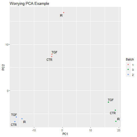
In the example image above the main source of variation is the batch in which the samples were sequenced. A multi-factor analysis to compare the various conditions, but “correct” for differences in batch, would be as follows.

### Don't run this. It's just a code example
design(MY_DATA) <- ~ batch + condition

Likewise, if we have different treatments applied to difference cell-lines, but the main source of variation is the cell line the following could be used.

### Don't run this. It's just a code example
design(MY_DATA) <- ~cell_line + treatment

Adding annotation to the DESeq2 results

We would love to share these results with our collaborators, or search for our favourite gene in the results. However, the results are not very useful in there current form as each row is named according to an Ensembl identifier. Whilst gene symbols are problematic and can change over time, they are the names that are most recognisable and make the results easier to navigate.

There are a number of ways to add annotation, but we will demonstrate how to do this using the org.Hs.eg.db package. This package is one of several organism-level packages in Bioconductor that are re-built every 6 months. These packages are listed on the annotation section of the Bioconductor, and are installed in the same way as regular Bioconductor packages. An alternative approach is to use biomaRt, an interface to the BioMart resource. BioMart is much more comprehensive, but the organism packages do not require online access once downloaded.

### Only execute when you need to install the package
install.packages("BiocManager")
BiocManager::install("org.Hs.eg.db")
# For Mouse
BiocManager::install("org.Mm.eg.db")

The packages are larger in size that Bioconductor software packages, but essentially they are databases that can be used to make offline queries. An alternatve (biomaRt) that connects to the ensembl biomart resource will be discussed later.

library(org.Hs.eg.db)

First we need to decide what information we want. In order to see what we can extract we can run the columns function on the annotation database.

columns(org.Hs.eg.db)

 [1] "ACCNUM"       "ALIAS"        "ENSEMBL"      "ENSEMBLPROT"  "ENSEMBLTRANS"
 [6] "ENTREZID"     "ENZYME"       "EVIDENCE"     "EVIDENCEALL"  "GENENAME"    
[11] "GENETYPE"     "GO"           "GOALL"        "IPI"          "MAP"         
[16] "OMIM"         "ONTOLOGY"     "ONTOLOGYALL"  "PATH"         "PFAM"        
[21] "PMID"         "PROSITE"      "REFSEQ"       "SYMBOL"       "UCSCKG"      
[26] "UNIPROT"

We are going to filter the database by a key or set of keys in order to extract the information we want. Valid names for the key can be retrieved with the keytypes function.

keytypes(org.Hs.eg.db)

 [1] "ACCNUM"       "ALIAS"        "ENSEMBL"      "ENSEMBLPROT"  "ENSEMBLTRANS"
 [6] "ENTREZID"     "ENZYME"       "EVIDENCE"     "EVIDENCEALL"  "GENENAME"    
[11] "GENETYPE"     "GO"           "GOALL"        "IPI"          "MAP"         
[16] "OMIM"         "ONTOLOGY"     "ONTOLOGYALL"  "PATH"         "PFAM"        
[21] "PMID"         "PROSITE"      "REFSEQ"       "SYMBOL"       "UCSCKG"      
[26] "UNIPROT"

We should see ENSEMBL, which is the type of key we are going to use in this case. If we are unsure what values are acceptable for the key, we can check what keys are valid with keys

keys(org.Hs.eg.db, keytype="ENSEMBL")[1:10]

 [1] "ENSG00000121410" "ENSG00000175899" "ENSG00000291190" "ENSG00000171428"
 [5] "ENSG00000156006" "ENSG00000196136" "ENSG00000114771" "ENSG00000127837"
 [9] "ENSG00000129673" "ENSG00000090861"

For the top gene in our analysis the call to the function would be:-

select(org.Hs.eg.db, keys=top_up,
       keytype = "ENSEMBL",columns=c("SYMBOL","GENENAME")
)

Unfortunately, the authors of dplyr and AnnotationDbi have both decided to use the name select in their packages. To avoid confusion and errors, the following code is sometimes used:-

AnnotationDbi::select(org.Hs.eg.db, keys=top_up,keytype = "ENSEMBL",columns=c("SYMBOL","GENENAME"))

'select()' returned 1:1 mapping between keys and columns

          ENSEMBL SYMBOL
1 ENSG00000119681  LTBP2
                                                  GENENAME
1 latent transforming growth factor beta binding protein 2

To annotate our results, we definitely want gene symbols and perhaps the full gene name. Let’s build up our annotation information into a new data frame using the select function.

anno <- AnnotationDbi::select(org.Hs.eg.db,keys=rownames(dds),
              columns=c("SYMBOL","GENENAME"),
              keytype="ENSEMBL")

'select()' returned 1:many mapping between keys and columns

# Have a look at the annotation
head(anno)

          ENSEMBL SYMBOL
1 ENSG00000000003 TSPAN6
2 ENSG00000000005   TNMD
3 ENSG00000000419   DPM1
4 ENSG00000000457  SCYL3
5 ENSG00000000460  FIRRM
6 ENSG00000000938    FGR
                                                     GENENAME
1                                               tetraspanin 6
2                                                 tenomodulin
3 dolichyl-phosphate mannosyltransferase subunit 1, catalytic
4                                    SCY1 like pseudokinase 3
5   FIGNL1 interacting regulator of recombination and mitosis
6              FGR proto-oncogene, Src family tyrosine kinase

However, we have a problem that the resulting data frame has more rows than our results table. This is due to the one-to-many relationships that often occur when mapping between various identifiers.

dim(anno)

[1] 58969     3

dim(dds)

[1] 57914     9

Such duplicated entries can be identified using the duplicated function. Fortunately, there are not too many so hopefully we won’t lose too much information if we discard the entries that are duplicated. The first occurrence of the duplicated ID will still be included in the table.

anno <- AnnotationDbi::select(org.Hs.eg.db,keys=rownames(dds),
            columns=c("ENSEMBL","SYMBOL","GENENAME","ENTREZID"),
            keytype="ENSEMBL") %>% 
filter(!duplicated(ENSEMBL))

'select()' returned 1:many mapping between keys and columns

dim(anno)

[1] 57914     4

We can bind in the annotation information to the results data frame.

results_annotated <- results(de_condition,tidy=TRUE) %>% 
  left_join(anno, by=c("row"="ENSEMBL")) %>% 
  arrange(padj)

head(results_annotated)

              row    baseMean log2FoldChange      lfcSE     stat        pvalue
1 ENSG00000119681   6471.7058       2.372065 0.07076496 33.52033 2.437260e-246
2 ENSG00000120708  22001.6982       1.436637 0.05904590 24.33084 9.248277e-131
3 ENSG00000172061   1481.6147       2.384971 0.09843523 24.22883 1.105455e-129
4 ENSG00000049540    932.0366       3.999465 0.17556867 22.78006 7.228861e-115
5 ENSG00000060718   1512.0092       2.123432 0.09532775 22.27506 6.448803e-110
6 ENSG00000115414 683348.5240       1.453310 0.06867840 21.16109  2.181368e-99
           padj  SYMBOL
1 4.371957e-242   LTBP2
2 8.294780e-127   TGFBI
3 6.609883e-126  LRRC15
4 3.241783e-111     ELN
5 2.313573e-106 COL11A1
6  6.521564e-96     FN1
                                                  GENENAME ENTREZID
1 latent transforming growth factor beta binding protein 2     4053
2                  transforming growth factor beta induced     7045
3                        leucine rich repeat containing 15   131578
4                                                  elastin     2006
5                           collagen type XI alpha 1 chain     1301
6                                            fibronectin 1     2335

We can save the results table using the write.csv function, which writes the results out to a csv file that you can open in excel.

write.csv(results_annotated,file="de_analysis/condition_TGF_vs_CTR_DESeq_annotated.csv",row.names=FALSE)

Exercise

The publication gives examples of COL1A1, COL1A2 and COL3A1 as genes that are up-regulated in TGF-treated samples vs controls (Figure 6C). Use your data to verify this by
1. extracting their p-values
2. plotting the counts for these genes

Solution

We already have the differential expression statistics for the contrast TGF vs CTR and have just added gene names (SYMBOL) into the results_annotated. We can therefore filter our results to rows that match any of these genes of interest.

genes_of_interest <- c("COL1A1", "COL1A2", "COL3A1")

## To make the output a bit cleaner I will select a few columns of interest. 
filter(results_annotated, SYMBOL %in% genes_of_interest) %>% 
  dplyr::select(log2FoldChange, padj, SYMBOL)

  log2FoldChange         padj SYMBOL
1      1.4077294 4.902831e-44 COL1A1
2      0.4442566 6.458329e-08 COL1A2
3      0.3552021 9.398496e-05 COL3A1

Indeed they all are significant with a positive fold-change indicating higher expression in TGF-treated samples. Plotting the counts for genes requires a bit more thought, as the following does not work as we might hope

plotCounts(dds, "COL1A1", intgroup = "condition")

`Error in counts(dds, normalized = normalized, replaced = replaced)[gene,  : 
  subscript out of bounds`

The error is not particularly helpful, but it basically means that it cannot find counts for COL1A1 in the dds object. Although we have added gene names to the analysis, they only appear in our results table and the gene counts are still referred to by ensembl IDS.

ens_ids <- filter(results_annotated, SYMBOL %in% genes_of_interest) %>% 
  pull(row)

ens_ids

[1] "ENSG00000108821" "ENSG00000164692" "ENSG00000168542"

This code works, but is a bit clunky. N.B. par(mfrow=c(1,3)) is the base R plotting way of making a panel with one row and three columns

par(mfrow=c(1,3))

plotCounts(dds, ens_ids[1], intgroup = "condition")
plotCounts(dds, ens_ids[2], intgroup = "condition")
plotCounts(dds, ens_ids[3], intgroup = "condition")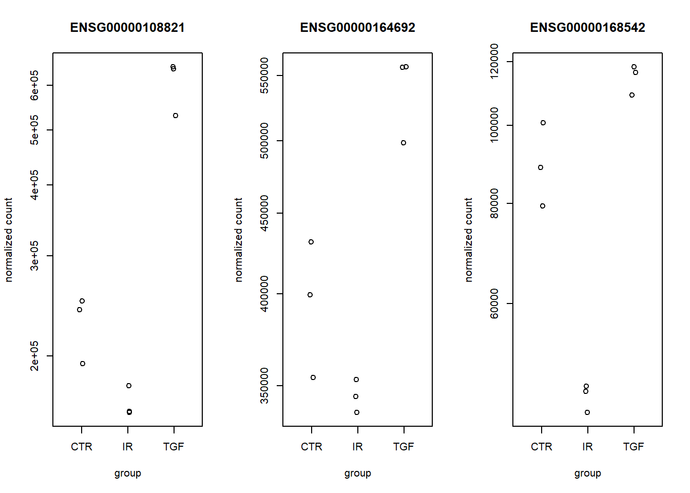

To do a nicer job we can use ggplot2 after some data manipulation. The first step is to get normalized counts for all genes after explicitly using the estimateSizeFactors. We don’t normally need to use this function as it is part of the DESeq workflow.

The results is a data frame with ensembl IDs in the rows.

dds <- estimateSizeFactors(dds)
norm_counts <- counts(dds, normalized = TRUE)
head(norm_counts)

                 1_CTR_BC_2  2_TGF_BC_4  3_IR_BC_5  4_CTR_BC_6   5_TGF_BC_7
ENSG00000000003 1496.753711 1309.582900 1503.06012 1550.428865 1326.3138781
ENSG00000000005    0.000000    0.000000    0.00000    0.000000    0.0000000
ENSG00000000419 1681.596633 1502.591885 2089.94798 1645.965855 1826.4150250
ENSG00000000457  661.642869  522.309405  673.12901  666.939177  629.4048655
ENSG00000000460  233.186455  261.577968  129.92174  203.812245  242.4444723
ENSG00000000938    9.479124    4.232653   12.32016    5.459257    0.9507626
                 6_IR_BC_12 7_CTR_BC_13 8_TGF_BC_14  9_IR_BC_15
ENSG00000000003 1465.288919  1639.42512 1287.173576 1297.038521
ENSG00000000005    0.000000     0.00000    0.000000    1.022095
ENSG00000000419 2058.823670  1893.34636 1392.402365 2023.748047
ENSG00000000457  622.515941   791.26495  557.148855  641.875643
ENSG00000000460  125.198737   258.13570  271.527857  129.806062
ENSG00000000938    2.318495    20.01869    3.758171    8.176760

We can filter these counts by the ensembl IDs we identified for these genes; provided that the ensembl ID appears as a column name.

norm_counts %>% 
  data.frame() %>% 
  tibble:::rownames_to_column("row") %>% 
  filter(row %in% ens_ids)

              row X1_CTR_BC_2 X2_TGF_BC_4 X3_IR_BC_5 X4_CTR_BC_6 X5_TGF_BC_7
1 ENSG00000108821    250216.6    646241.5  158906.61   241050.74    530262.2
2 ENSG00000164692    431598.7    556886.8  344485.25   399621.22    498829.0
3 ENSG00000168542    100729.0    118220.5   46646.38    88590.09    109123.8
  X6_IR_BC_12 X7_CTR_BC_13 X8_TGF_BC_14 X9_IR_BC_15
1   159665.49    193788.27     641086.7   177323.26
2   336490.15    354051.56     556982.6   353092.93
3    47357.58     79414.13     116412.2    43879.56

However, these are not in the tidy form that ggplot2 requires so we have to reshape the data using tidyr’s pivot_longer function. Turning the counts into a data frame introduced an “X” at the start of the column names, so we better remove that.

norm_counts %>% 
  data.frame() %>% 
  tibble:::rownames_to_column("row") %>% 
  filter(row %in% ens_ids) %>% 
  tidyr::pivot_longer(-row, names_to = "Run", values_to = "count") %>% 
  mutate(Run = stringr::str_remove_all(Run, "X"))

# A tibble: 27 × 3
   row             Run           count
   <chr>           <chr>         <dbl>
 1 ENSG00000108821 1_CTR_BC_2  250217.
 2 ENSG00000108821 2_TGF_BC_4  646241.
 3 ENSG00000108821 3_IR_BC_5   158907.
 4 ENSG00000108821 4_CTR_BC_6  241051.
 5 ENSG00000108821 5_TGF_BC_7  530262.
 6 ENSG00000108821 6_IR_BC_12  159665.
 7 ENSG00000108821 7_CTR_BC_13 193788.
 8 ENSG00000108821 8_TGF_BC_14 641087.
 9 ENSG00000108821 9_IR_BC_15  177323.
10 ENSG00000164692 1_CTR_BC_2  431599.
# ℹ 17 more rows

Now we have the counts in a tidy form, but we don’t know the sample groupings. The groupings can be obtained from the colData

sampleInfo <- colData(dds) %>% data.frame

norm_counts %>% 
  data.frame() %>% 
  tibble:::rownames_to_column("row") %>% 
  filter(row %in% ens_ids) %>% 
  tidyr::pivot_longer(-row, names_to = "Run", values_to = "count") %>% 
  mutate(Run = stringr::str_remove_all(Run, "X")) %>% 
  left_join(sampleInfo, by = "Run")

# A tibble: 27 × 8
   row             Run        count condition Name  Replicate Treated sizeFactor
   <chr>           <chr>      <dbl> <fct>     <chr>     <int> <chr>        <dbl>
 1 ENSG00000108821 1_CTR_BC… 2.50e5 CTR       CTR_1         1 N            1.05 
 2 ENSG00000108821 2_TGF_BC… 6.46e5 TGF       TGF_1         1 Y            1.18 
 3 ENSG00000108821 3_IR_BC_5 1.59e5 IR        IR_1          1 Y            0.893
 4 ENSG00000108821 4_CTR_BC… 2.41e5 CTR       CTR_2         2 N            1.10 
 5 ENSG00000108821 5_TGF_BC… 5.30e5 TGF       TGF_2         2 Y            1.05 
 6 ENSG00000108821 6_IR_BC_… 1.60e5 IR        IR_2          2 Y            0.863
 7 ENSG00000108821 7_CTR_BC… 1.94e5 CTR       CTR_3         3 N            0.949
 8 ENSG00000108821 8_TGF_BC… 6.41e5 TGF       TGF_3         3 Y            1.06 
 9 ENSG00000108821 9_IR_BC_… 1.77e5 IR        IR_3          3 Y            0.978
10 ENSG00000164692 1_CTR_BC… 4.32e5 CTR       CTR_1         1 N            1.05 
# ℹ 17 more rows

Finally, we can make the plot of count against condition

library(ggplot2)
norm_counts %>% 
  data.frame() %>% 
  tibble:::rownames_to_column("row") %>% 
  filter(row %in% ens_ids) %>% 
  tidyr::pivot_longer(-row, names_to = "Run", values_to = "count") %>% 
  mutate(Run = stringr::str_remove_all(Run, "X")) %>% 
  left_join(sampleInfo, by = "Run") %>% 
  ggplot(aes(x = condition, y = count, col = condition)) + geom_jitter(width=0.1) + facet_wrap(~row)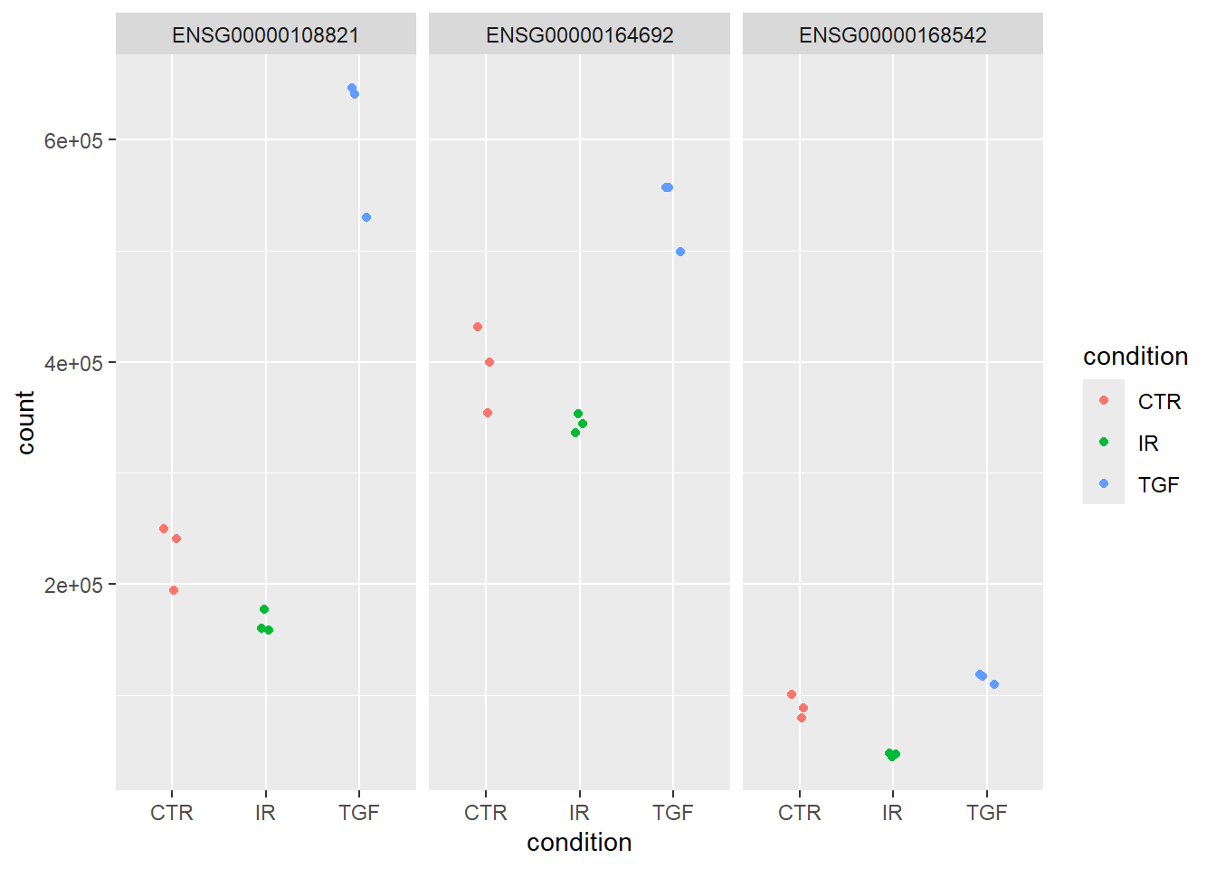

But what are the most recognisable names for these genes? We could use the results_annotated table that we already made and we could then facet using the SYMBOL which will print the gene names automatically.

norm_counts %>% 
  data.frame() %>% 
  tibble:::rownames_to_column("row") %>% 
  filter(row %in% ens_ids) %>% 
  tidyr::pivot_longer(-row, names_to = "Run", values_to = "count") %>% 
  mutate(Run = stringr::str_remove_all(Run, "X")) %>% 
  left_join(sampleInfo, by = "Run") %>% 
  left_join(results_annotated, by = "row") %>% 
  ggplot(aes(x = condition, y = count, col = condition)) + geom_jitter(width=0.1) + facet_wrap(~SYMBOL)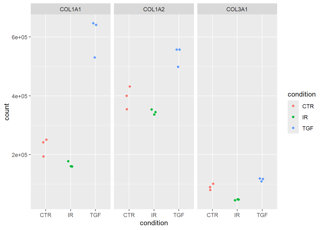

Admittedly, that was quite a bit of effort and would have been simpler with a tidybulk approach from the start. If you were interested in lots of gene sets like genes_of_interest then it would we worth making the code into a function that could be run without having to repeat the code all the time.

Heatmaps

You may have already seen the use of a heatmap as a quality assessment tool to visualise the relationship between samples in an experiment. Another common use-case for such a plot is to visualise the results of a differential expression analysis. Although ggplot2 has a geom_tile function to make heatmaps, specialised packages such as pheatmaps offer more functionality such as clustering the samples.

The counts we are visualising are the variance-stablised counts, which are more appropriate for visualisation.

Here we will take the top 10 genes from the differential expression analysis and produce a heatmap with the pheatmap package. We can take advantage of the fact the our counts table contains Ensembl gene names in the rows. Standard subset operations in R can then be used.

The default colour palette goes from low expression in blue to high expression in red, which is a good alternative to the traditional red/green heatmaps which are not suitable for those with forms of colour-blindness.

# pheatmap is a specialised package to make heatmaps
library(pheatmap)
top_genes <- dplyr::slice_min(results_annotated, padj, n = 10) %>% pull(row)
vsd <- vst(dds)

# top_genes is a vector containing ENSEMBL names of the genes we want to see in the heatmap

pheatmap(assay(vsd)[top_genes,])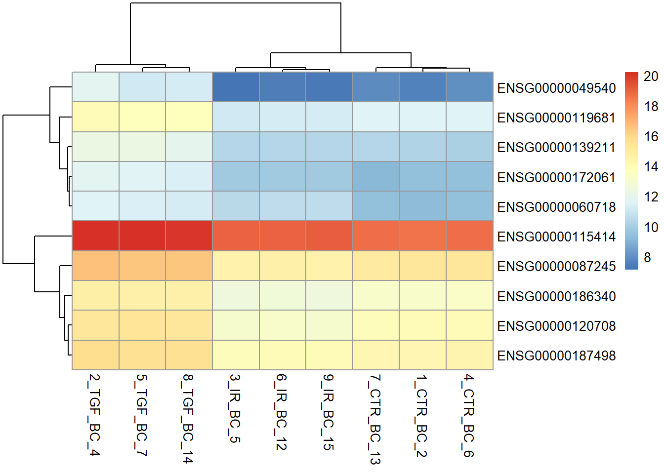

The heatmap is more informative if we add colours underneath the sample dendrogram to indicate which sample group each sample belongs to. This we can do by creating a data frame containing metadata for each of the samples in our dataset. With the DESeq2 workflow we have already created such a data frame. We have to make sure the the rownames of the data frame are the same as the column names of the counts matrix.

Expression patterns are also easier to discern if we use scale = TRUE, which scales each gene (row) using the average expression level. Thus, we can now see which individual samples the gene is up- or down-regulated in.

sampleInfo <- as.data.frame(colData(dds)[,c("condition","Treated")])

pheatmap(assay(vsd)[top_genes,],
         annotation_col = sampleInfo,
         scale="row")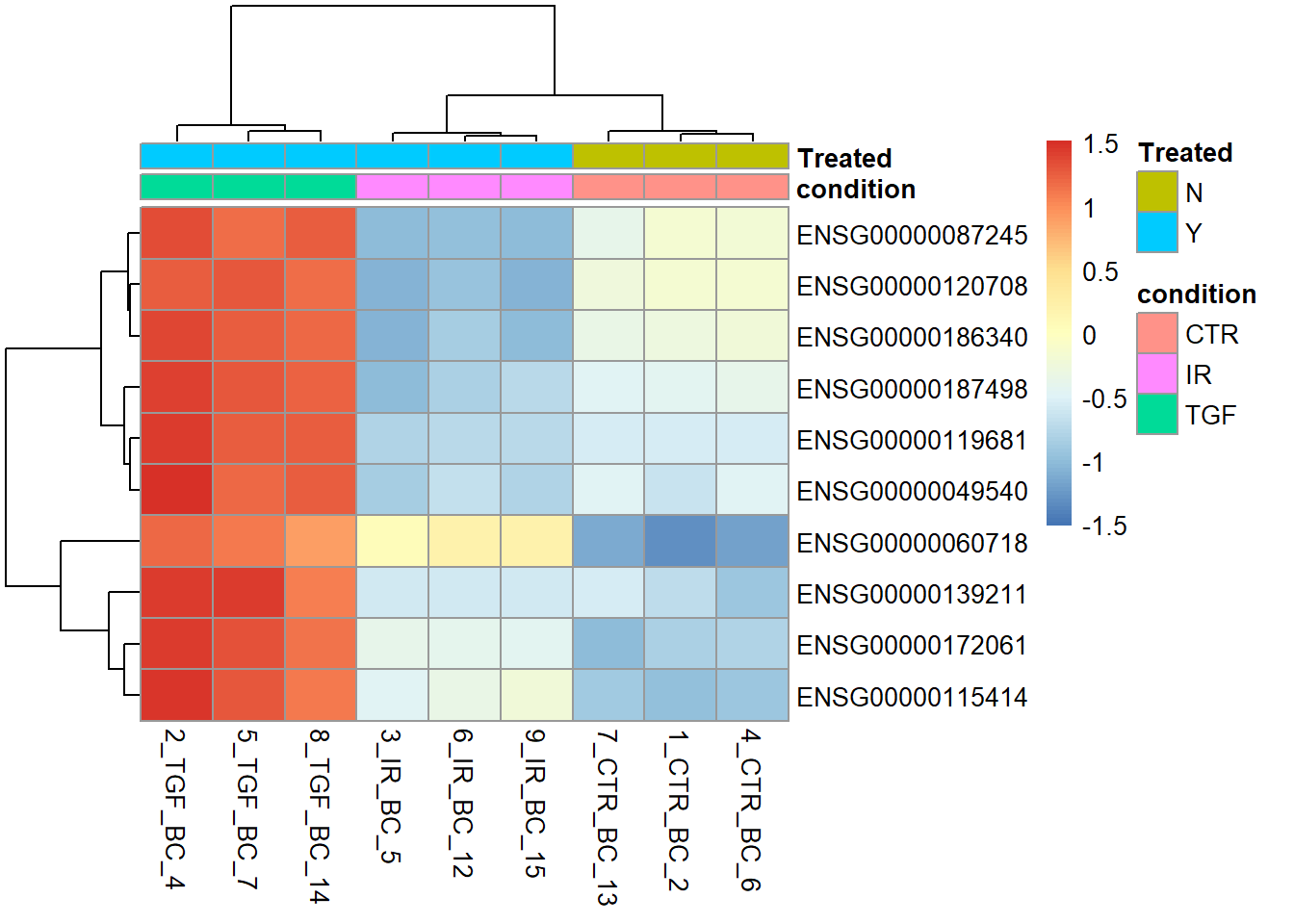

Any plot we create in RStudio can be saved as a png or pdf file. We use the png or pdf function to create a file for the plot to be saved into and run the rest of the code as normal. The plot does not get displayed in RStudio, but printed to the specified file.

png("heatmap_top10_genes.png",width=800,height=800)
pheatmap(assay(vsd)[top_genes,],
         annotation_col = sampleInfo,
         scale = "row")

There are many arguments to explore in pheatmap. A useful option is to specific our own labels for the rows (genes). The default is to use the rownames of the count matrix. In our case these are ENSEMBL IDs and not easy to interpret.

N <- 10
gene_labels <- dplyr::slice_min(results_annotated, padj, n = 10) %>% pull(SYMBOL)

pheatmap(assay(vsd)[top_genes,],
         annotation_col = sampleInfo,
         labels_row = gene_labels,
         scale="row")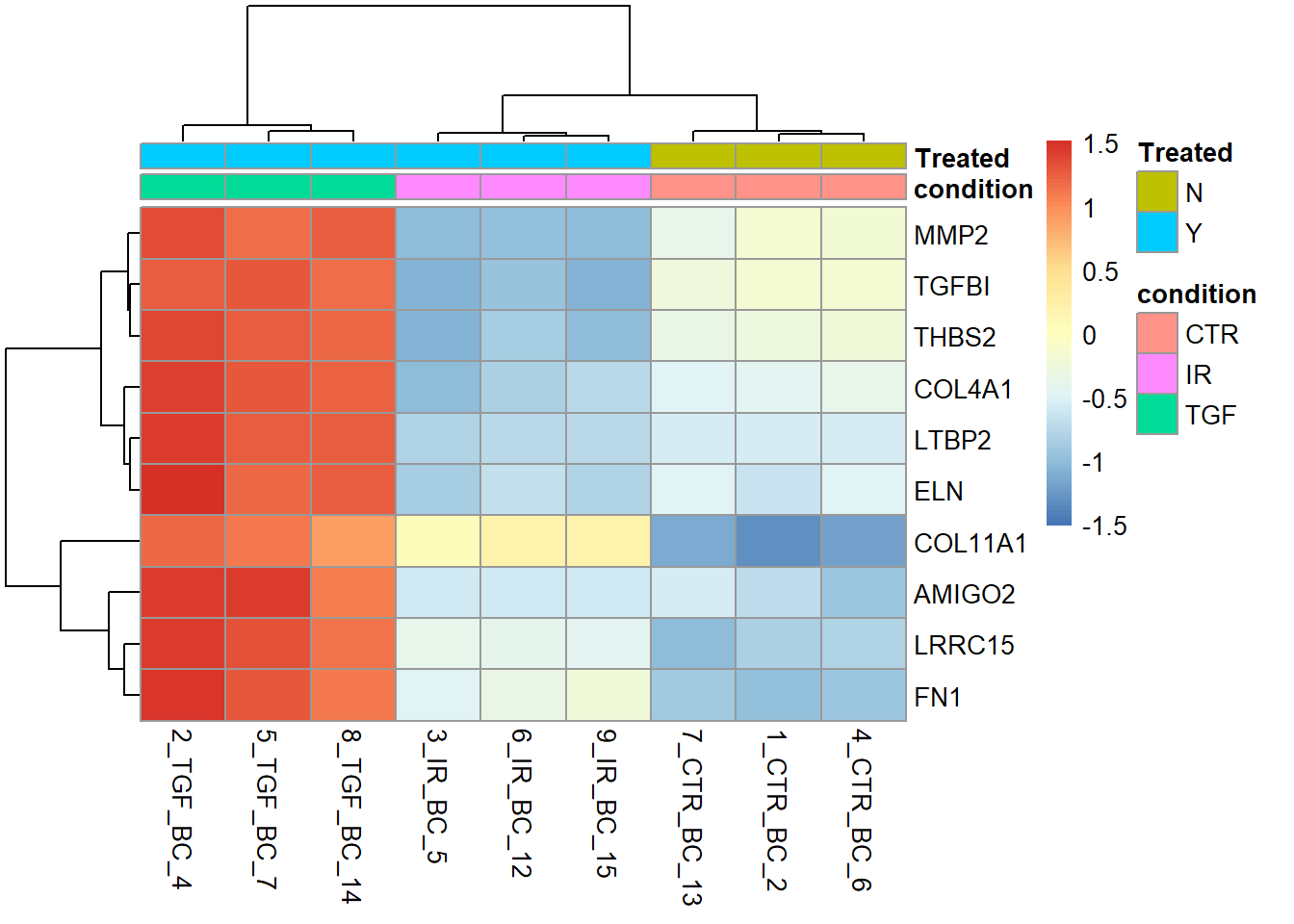

Since we are only interested in CTR and TGF samples for this analysis it might make sense not to include the IR samples in the plot (however, I personally like to include all samples to get a better impression of the data variability). The matrix we use as an argument to pheatmap can be subset accordingly, for example by creating a vector that contains only the indices of the CTR and TGF samples

no_ir <- which(dds$condition != "IR")

pheatmap(assay(vsd)[top_genes,no_ir],
         annotation_col = sampleInfo[no_ir,],scale="row")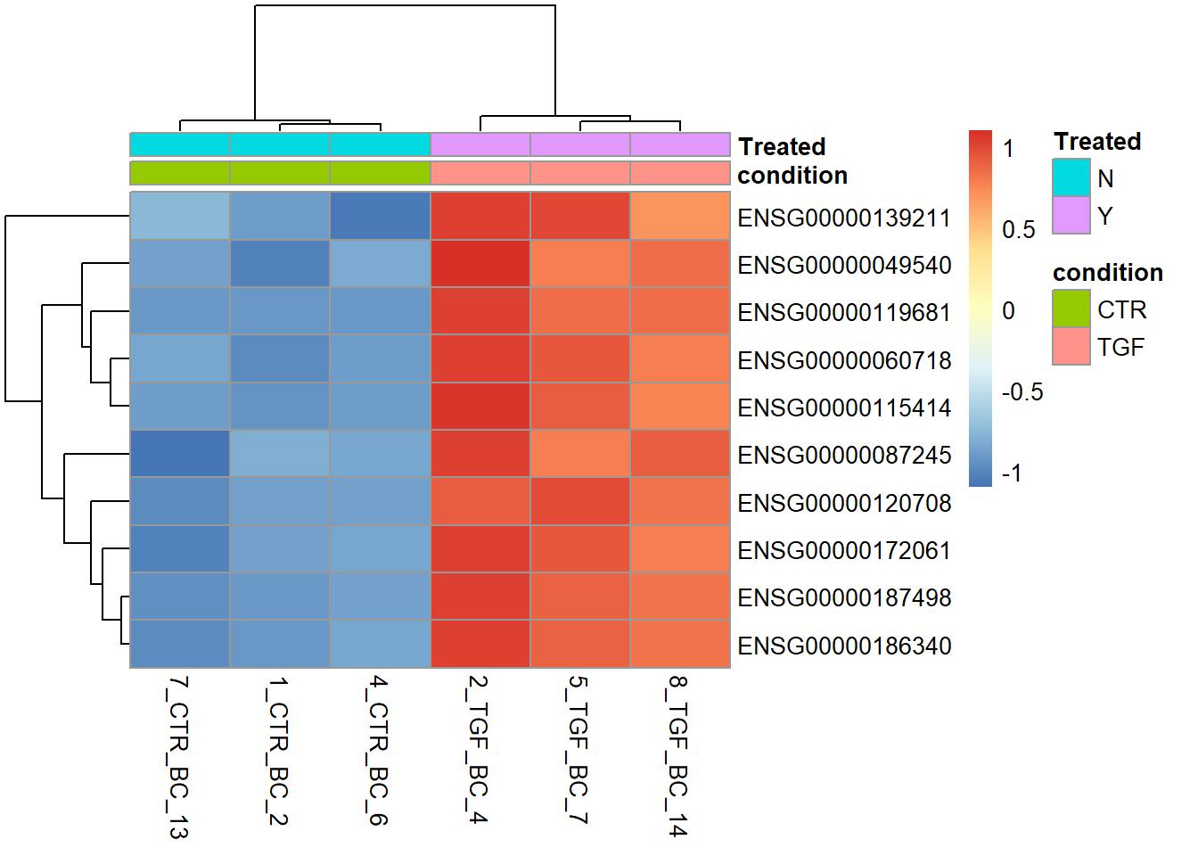

The clustering of columns (or indeed rows) can also be turned off.

pheatmap(assay(vsd)[top_genes,no_ir],
         annotation_col = sampleInfo[no_ir,],
         scale = "row",
         cluster_cols = FALSE)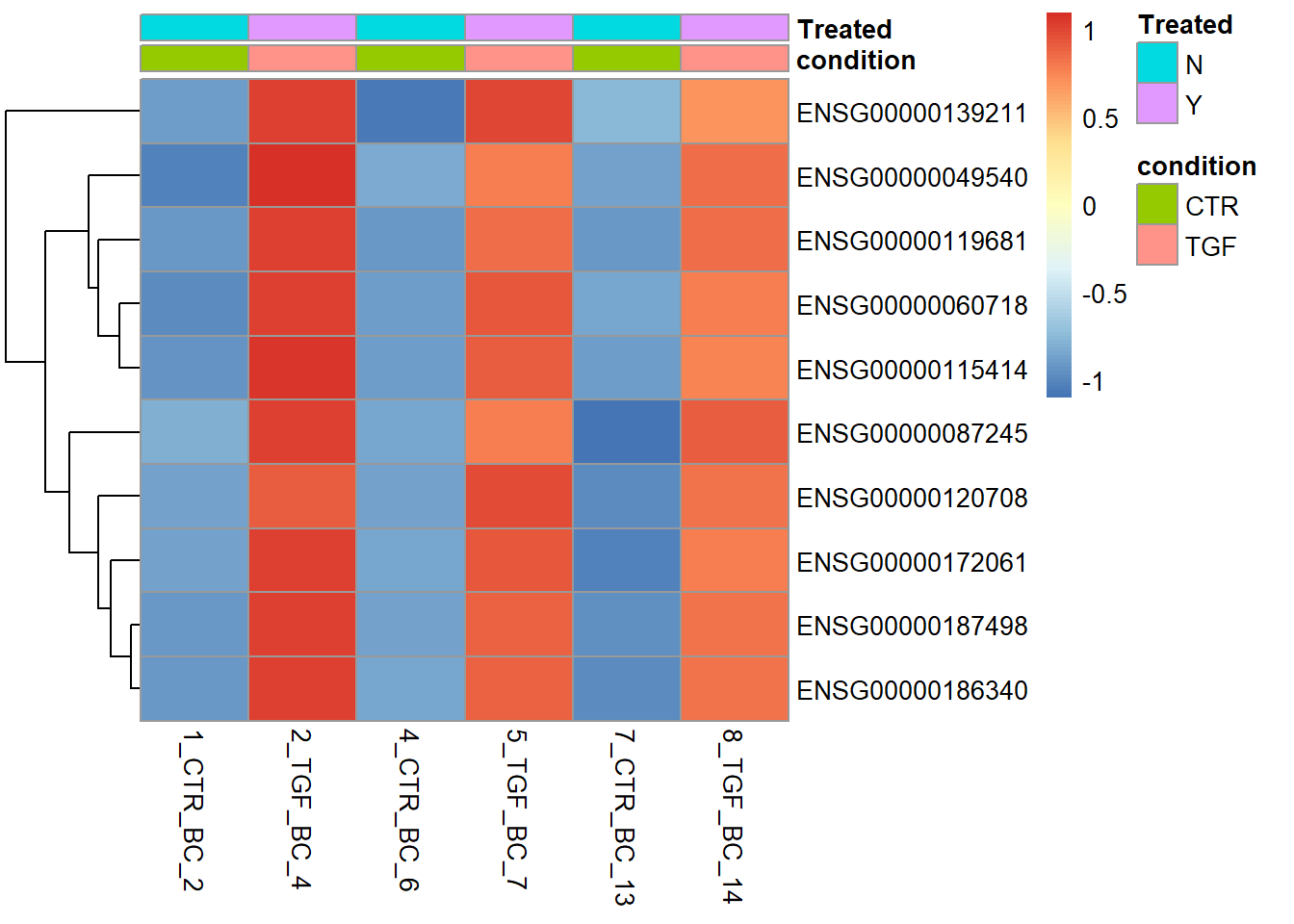

Given the nature of how the genes were selected for the heatmap (i.e. picking the most statistically significant), we shouldn’t be surprised by the good separation that it demonstrates. Another use we will see later on is for a gene list of our choosing relating to a particular biological pathway.

Exercise

Produce a heatmap using the top 30 genes with the most extreme log2 Fold-Change
- HINT: The abs function can be used to convert all negative values to positive.
Label the heatmap with the gene SYMBOL of the genes
Is this heatmap as effective as separating the samples into groups?

Solution

top_genes <-dplyr::slice_max(results_annotated, abs(log2FoldChange), n = 30) %>% 
  pull(row)

labels <- dplyr::slice_max(results_annotated, abs(log2FoldChange), n = 30) %>% 
  pull(SYMBOL)

sampleInfo <- as.data.frame(colData(dds)[,c("condition","Treated")])


pheatmap(assay(vsd)[top_genes,],
         scale= "row",
         annotation_col = sampleInfo, 
         labels_row = labels)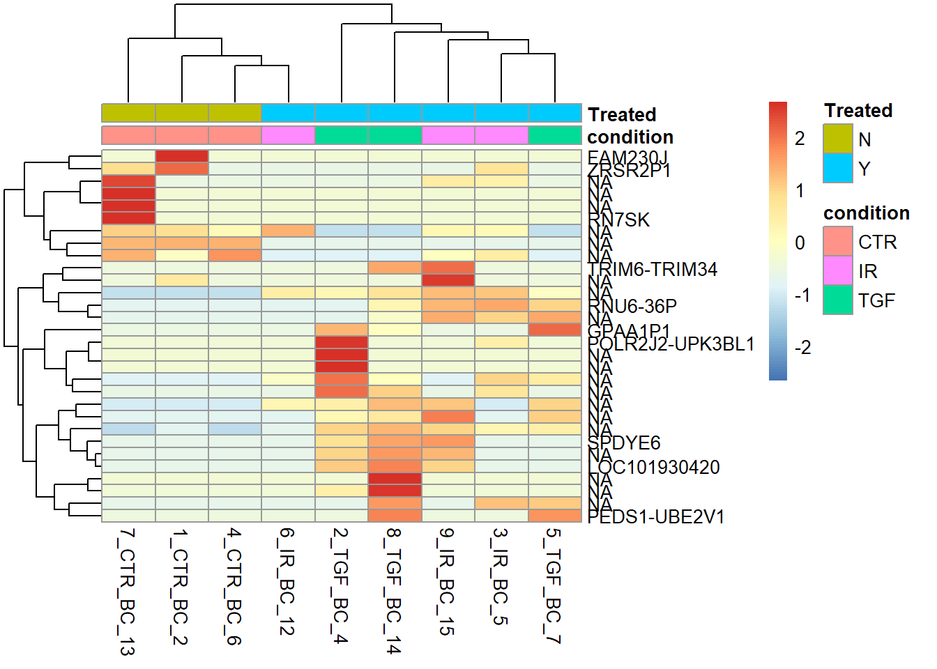

The samples are not cleanly separated when LFC is used, as it looks like the large LFC values are driven by outliers in a single sample. Most of the gene names are not recognisable to me, or NA, making me suspicious that these are just random findings.

ComplexHeatmap

Although I haven’t personally used it, the ComplexHeatmap is another popular choice for heatmaps of biological data. It promises more flexibility than pheatmap and support for multi-layered plot and is particularly useful for multi-omics and single-cell data

ComplexHeatmap

The volcano plot

The last visualisation we will cover in this section is the volcano plot which is another way of looking at all your results. Similar to the MA plot, it shows the log2FoldChange on the x-axis and the statistical significance is shown so that the most significant genes are the highest on the y-axis.

It’s perfectly possible to make this plot using standard ggplot2 commands, but the package EnhancedVolcano does a really good job out of the box. If you don’t have EnhancedVolcano installed you can use the following code:-

if(!require(BiocManager)) install.packages("BiocManager")
if(!require(EnhancedVolcano)) BiocManager::install("EnhancedVolcano")

EnhancedVolcano is useful as it will automatically label the names of the most significant genes and apply a colour scheme.

library(EnhancedVolcano)

EnhancedVolcano(results_annotated, x = "log2FoldChange", 
                y = "padj", 
                lab = results_annotated$SYMBOL, 
                title = "TGF vs CTRL",
                subtitle = "")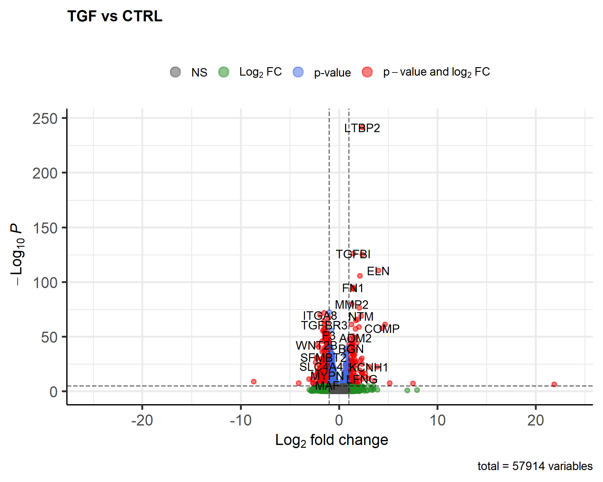

This is quite a nice result using the defaults. As the function is using ggplot2 under the hood it can be saved in the same ways as ordinary ggplot2 figures.

ggsave("TGF_vs_CTR_volcano.png")

Saving 7 x 5 in image

Rather than labeling all the genes, we can just highlight some of interest

EnhancedVolcano(results_annotated, x = "log2FoldChange", 
                y = "padj", 
                lab = results_annotated$SYMBOL, 
                title = "TGF vs CTRL",
                selectLab = genes_of_interest,
                drawConnectors = TRUE,
                FCcutoff = 0.5,
                pCutoff = 0.05,
                subtitle  = "Selected ECM Genes")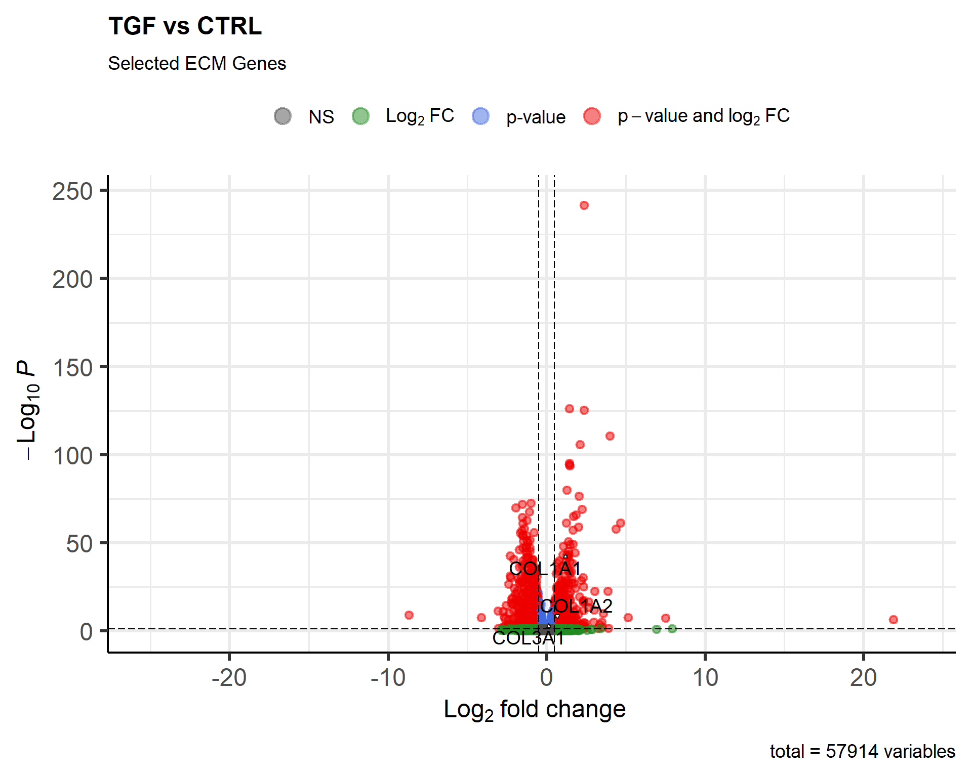

Exporting normalized counts

The DESeq workflow applies median of ratios normalization that accounts for differences in sequencing depth between samples. The user does not usually need to run this step. However, if you want a matrix of counts for some application outside of Bioconductor the values can be extracted from the dds object.

dds <- estimateSizeFactors(dds) 
countMatrix <-counts(dds, normalized=TRUE) 
head(countMatrix)

                 1_CTR_BC_2  2_TGF_BC_4  3_IR_BC_5  4_CTR_BC_6   5_TGF_BC_7
ENSG00000000003 1496.753711 1309.582900 1503.06012 1550.428865 1326.3138781
ENSG00000000005    0.000000    0.000000    0.00000    0.000000    0.0000000
ENSG00000000419 1681.596633 1502.591885 2089.94798 1645.965855 1826.4150250
ENSG00000000457  661.642869  522.309405  673.12901  666.939177  629.4048655
ENSG00000000460  233.186455  261.577968  129.92174  203.812245  242.4444723
ENSG00000000938    9.479124    4.232653   12.32016    5.459257    0.9507626
                 6_IR_BC_12 7_CTR_BC_13 8_TGF_BC_14  9_IR_BC_15
ENSG00000000003 1465.288919  1639.42512 1287.173576 1297.038521
ENSG00000000005    0.000000     0.00000    0.000000    1.022095
ENSG00000000419 2058.823670  1893.34636 1392.402365 2023.748047
ENSG00000000457  622.515941   791.26495  557.148855  641.875643
ENSG00000000460  125.198737   258.13570  271.527857  129.806062
ENSG00000000938    2.318495    20.01869    3.758171    8.176760

write.csv(countMatrix,file="normalized_counts.csv")

Let’s wrap-up for now and continue our exploration of the differential expression in the next section. If you want to find out more about the DESeq workflow then read on.

Full DESeq workflow

The median of ratios normalisation method is employed in DESeq2 to account for sequencing depth and RNA composition. Let’s go through a short worked example (courtesy of https://hbctraining.github.io/DGE_workshop/lessons/02_DGE_count_normalization.html) to explain the process.

## create a small example matrix of "counts"
test_data <- matrix(c(1489,22,793,76,521,906,13,410,42,1196),nrow=5)
rownames(test_data) <- c("EF2A","ABCD1","MEFV","BAG1","MOV10")
colnames(test_data) <- c("SampleA","SampleB")
test_data

      SampleA SampleB
EF2A     1489     906
ABCD1      22      13
MEFV      793     410
BAG1       76      42
MOV10     521    1196

Firstly, an “average” or reference sample is created that represents the counts on a typical sample in the dataset. The geometric mean is used rather than the arithmetic mean. In other words the individual counts are multiplied rather than summed and the measure should be more robust to outliers.

psuedo_ref <- sqrt(rowProds(test_data))
psuedo_ref

      EF2A      ABCD1       MEFV       BAG1      MOV10 
1161.47923   16.91153  570.20172   56.49779  789.37697

A ratios of sample to “psuedo reference” are then calculated for each gene. We are assuming that most genes are not changing dramatically, so this ratio should be somewhere around 1.

test_data/psuedo_ref

        SampleA   SampleB
EF2A  1.2819859 0.7800398
ABCD1 1.3008873 0.7687061
MEFV  1.3907359 0.7190438
BAG1  1.3451854 0.7433919
MOV10 0.6600142 1.5151189

DESeq2 defines size factors as being the median of these ratios for each sample (median is used so any outlier genes will not affect the normalisation).

norm_factors <- colMedians(test_data/psuedo_ref)
norm_factors

  SampleA   SampleB 
1.3008873 0.7687061

Individual samples can then normalised by dividing the count for each gene by the corresponding normalization factor.

test_data[,1] / norm_factors[1]

      EF2A      ABCD1       MEFV       BAG1      MOV10 
1144.60340   16.91153  609.58395   58.42166  400.49589

and for the second sample…

test_data[,2] / norm_factors[2]

      EF2A      ABCD1       MEFV       BAG1      MOV10 
1178.60387   16.91153  533.36378   54.63727 1555.86118

The size factors for each sample in our dataset can be calculated using the estimateSizeFactorsForMatrix function.

sf <- estimateSizeFactorsForMatrix(assay(dds))
sf

 1_CTR_BC_2  2_TGF_BC_4   3_IR_BC_5  4_CTR_BC_6  5_TGF_BC_7  6_IR_BC_12 
  1.0549498   1.1812922   0.8928452   1.0990507   1.0517872   0.8626285 
7_CTR_BC_13 8_TGF_BC_14  9_IR_BC_15 
  0.9491132   1.0643475   0.9783827

The estimation of these factors can also take gene-lengths into account, and this is implemented in the estimateSizeFactors function. Extra normalization factor data is added to the dds object.

dds <- estimateSizeFactors(dds)
dds

In preparation for differential expression DESeq2 also need a reliable estimate of the variability of each gene; which it calls dispersion.

dds <- estimateDispersions(dds)
dds

A statistical test can then be applied. As the data are count-based and not normally-distributed a t-test would not be appropriate. Most tests are based on a Poisson or negative-binomial distribution; negative binomial in the case of DESeq2. Although you might not be familiar with the negative binomial, the results should be in a familiar form with fold-changes and p-values for each gene.

dds <- nbinomWaldTest(dds)

It may seem like there is a lot to remember, but fortunately there is one convenient function that will apply the three steps (DESeq). The messages printed serve as reminders of the steps included.

Appendix: Annotation with the biomaRt resource

The Bioconductor package have the convenience of being able to make queries offline. However, they are only available for certain organisms. If your organism does not have an org.XX.eg.db package listed on the Bioconductor annotation page (http://bioconductor.org/packages/release/BiocViews.html#___AnnotationData), an alternative is to use biomaRt which provides an interface to the popular biomart annotation resource.

The first step is to find the name of a database that you want to connect to.

library(biomaRt)
listMarts()

               biomart                version
1 ENSEMBL_MART_ENSEMBL      Ensembl Genes 115
2   ENSEMBL_MART_MOUSE      Mouse strains 115
3     ENSEMBL_MART_SNP  Ensembl Variation 115
4 ENSEMBL_MART_FUNCGEN Ensembl Regulation 115

ensembl=useMart("ENSEMBL_MART_ENSEMBL")
# list the available datasets (species). Replace human with the name of your organism
listDatasets(ensembl) %>% dplyr::filter(grepl("Human",description))

                dataset              description    version
1 hsapiens_gene_ensembl Human genes (GRCh38.p14) GRCh38.p14

ensembl = useDataset("hsapiens_gene_ensembl", mart=ensembl)

Queries to biomaRt are constructed in a similar way to the queries we performed with the org.Hs.eg.db package. Instead of keys we have filters, and instead of columns we have attributes. The list of acceptable values is much more comprehensive that for the org.Hs.eg.db package.

listFilters(ensembl) %>% 
    dplyr::filter(grepl("ensembl",name))

                           name
1               ensembl_gene_id
2       ensembl_gene_id_version
3         ensembl_transcript_id
4 ensembl_transcript_id_version
5            ensembl_peptide_id
6    ensembl_peptide_id_version
7               ensembl_exon_id
                                                     description
1                       Gene stable ID(s) [e.g. ENSG00000000003]
2       Gene stable ID(s) with version [e.g. ENSG00000000003.17]
3                 Transcript stable ID(s) [e.g. ENST00000000233]
4 Transcript stable ID(s) with version [e.g. ENST00000000233.10]
5                    Protein stable ID(s) [e.g. ENSP00000000233]
6     Protein stable ID(s) with version [e.g. ENSP00000000233.5]
7                              Exon ID(s) [e.g. ENSE00000000001]

listAttributes(ensembl) %>% 
    dplyr::filter(grepl("gene",name)) %>% 
  slice_sample(n = 10)

                                     name
1                                  gene3d
2    cldingo_homolog_associated_gene_name
3     cgpicr_homolog_associated_gene_name
4         platipinna_homolog_ensembl_gene
5                    external_gene_source
6  osinensis_homolog_associated_gene_name
7     psimus_homolog_associated_gene_name
8         ogarnettii_homolog_ensembl_gene
9     oaries_homolog_associated_gene_name
10          cporosus_homolog_ensembl_gene
                                     description         page
1                                      Gene3D ID feature_page
2                                Dingo gene name     homologs
3                 Chinese hamster PICR gene name     homologs
4                   Sailfin molly gene stable ID     homologs
5                            Source of gene name  snp_somatic
6                       Chinese medaka gene name     homologs
7                 Greater bamboo lemur gene name     homologs
8                        Bushbaby gene stable ID     homologs
9                                Sheep gene name     homologs
10 Australian saltwater crocodile gene stable ID     homologs

An advantage over the org.. packages is that positional information can be retrieved

attributeNames <- c('ensembl_gene_id', 'entrezgene_id', 'external_gene_name', "chromosome_name","start_position","end_position")

top_genes <- results_annotated %>% 
  slice_min(padj, n = 10) %>% 
  pull(row)

getBM(attributes = attributeNames,
      filters = "ensembl_gene_id",
      values= top_genes,
      mart=ensembl)

   ensembl_gene_id entrezgene_id external_gene_name chromosome_name
1  ENSG00000049540          2006                ELN               7
2  ENSG00000060718          1301            COL11A1               1
3  ENSG00000087245          4313               MMP2              16
4  ENSG00000115414          2335                FN1               2
5  ENSG00000119681          4053              LTBP2              14
6  ENSG00000120708          7045              TGFBI               5
7  ENSG00000139211        347902             AMIGO2              12
8  ENSG00000172061        131578             LRRC15               3
9  ENSG00000186340          7058              THBS2               6
10 ENSG00000187498          1282             COL4A1              13
   start_position end_position
1        74027789     74069909
2       102876467    103108872
3        55389700     55506691
4       215360440    215436120
5        74498183     74612378
6       136028988    136063818
7        47075707     47080902
8       194355249    194369743
9       169215780    169254060
10      110148963    110307202

Quick Start

Differential expression with DESeq2

Recap of pre-processing

The DESeq workflow in brief

Processing the DE results using tidyverse

Changing the direction of the contrast, or the groups being compared

Exercise

More complex designs

Adding annotation to the DESeq2 results

Exercise

Heatmaps

Exercise

The volcano plot

Exporting normalized counts

Full DESeq workflow

Appendix: Annotation with the biomaRt resource

Differential expression with `DESeq2`