Introduction to R - Part 1

Overview

In these materials, we explore fundamental operations of R and load some example data

Topics Covered

• Basic calculations in R
• Using functions
• Getting help
• Saving data using variables
• Reading a spreadsheet into R

Setup

If you are following these notes independently (outside one of our workshops)

From the RStudio menus, Choose the File -> New Project option and select New Directory from the new window

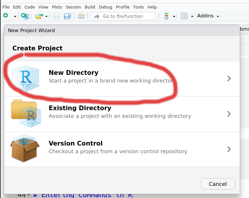
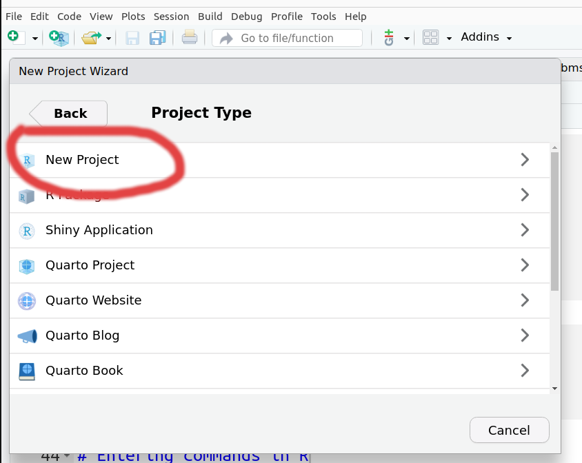
Then for the Project Type pick New Project.

It will ask you to pick a new Directory name, and where to create that directory (e.g. your Home directory or directory where you usually save your work)

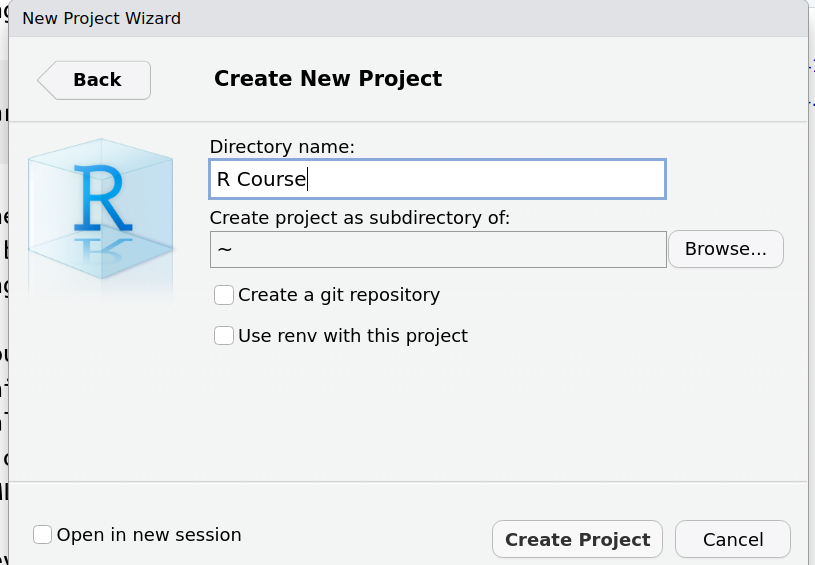
RStudio should now refresh itself. You can now download the data required for the workshop by copying and pasting the following into the R console (as shown in the screenshot)

dir.create("raw_data/",showWarnings = FALSE)
download.file("https://raw.githubusercontent.com/markdunning/markdunning.github.com/refs/heads/master/files/training/r/raw_data/gapminder.csv", destfile = "raw_data/gapminder.csv")

You will need to install some R packages and download some data before you start. You can install the packages by copying and pasting the following into an R console and pressing ENTER

install.packages("dplyr")
install.packages("ggplot2")
install.packages("readr")
install.packages("rmarkdown")
install.packages("tidyr")

You can check that this worked by copying and pasting the following:-

source("https://raw.githubusercontent.com/markdunning/markdunning.github.com/refs/heads/master/files/training/r/check_packages.R")

Attaching package: 'dplyr'

The following objects are masked from 'package:stats':

    filter, lag

The following objects are masked from 'package:base':

    intersect, setdiff, setequal, union

The dplyr package has been installed

The ggplot2 package has been installed

The readr package has been installed

The rmarkdown package has been installed

The tidyr package has been installed

You have successfully installed all the packages required for the course

Your output should be like that shown above - indicating that all required packages are present. 🎉We will cover the purpose of R packages to extend the default R functionality later.

However, we will not be working with the data or packages we downloaded just yet, as we need to cover some fundamentals first

Entering commands in R

The traditional way to enter R commands is via the Terminal, or using the console in RStudio (bottom-left panel when RStudio opens for first time). This doesn’t automatically keep track of the steps you did.

We’ll be working in an R Notebook. These file are an R Markdown document type, which allow us to combine R code with markdown, a documentation language, providing a framework for literate programming. In an R Notebook, R code chunks can be executed independently and interactively, with output visible immediately beneath the input.

Let’s try this now!

print("Hello World")

[1] "Hello World"

R can be used as a calculator to compute simple sums

2 + 2

[1] 4

2 - 2

[1] 0

4 * 3

[1] 12

10 / 2

[1] 5

The answer is displayed at the console with a [1] in front of it. The 1 inside the square brackets is a place-holder to signify how many values were in the answer (in this case only one). We will talk about dealing with lists of numbers shortly…

In the case of expressions involving multiple operations, R respects the BODMAS system to decide the order in which operations should be performed.

2 + 2 *3

[1] 8

2 + (2 * 3)

[1] 8

(2 + 2) * 3

[1] 12

R is capable of more complicated arithmetic such as trigonometry and logarithms; like you would find on a fancy scientific calculator. Of course, R also has a plethora of statistical operations as we will see.

pi

[1] 3.141593

sin (pi/2)

[1] 1

cos(pi)

[1] -1

tan(2)

[1] -2.18504

log(1)

[1] 0

We can only go so far with performing simple calculations like this. Eventually we will need to store our results for later use. For this, we need to make use of variables.

Variables

A variable is a letter or word which takes (or contains) a value. We use the assignment ‘operator’, <- to create a variable and store some value in it.

x <- 10
x

[1] 10

myNumber <- 25
myNumber

[1] 25

We also can perform arithmetic on variables using functions:

sqrt(myNumber)

[1] 5

We can add variables together:

x + myNumber

[1] 35

We can change the value of an existing variable:

x <- 21
x

[1] 21

We can set one variable to equal the value of another variable:

x <- myNumber
x

[1] 25

When we are feeling lazy we might give our variables short names (x, y, i…etc), but a better practice would be to give them meaningful names. There are some restrictions on creating variable names. They cannot start with a number or contain characters such as . and ‘-’. Naming variables the same as in-built functions in R, such as c, T, mean should also be avoided.

Naming variables is a matter of taste. Some conventions exist such as a separating words with - or using camelCaps. Whatever convention you decided, stick with it!

Functions

Functions in R perform operations on arguments (the inputs(s) to the function). We have already used:

sin(x)

[1] -0.1323518

this returns the sine of x. In this case the function has one argument: x. Arguments are always contained in parentheses – curved brackets, () – separated by commas.

Arguments can be named or unnamed, but if they are unnamed they must be ordered (we will see later how to find the right order). The names of the arguments are determined by the author of the function and can be found in the help page for the function. When testing code, it is easier and safer to name the arguments. seq is a function for generating a numeric sequence from and to particular numbers. Type ?seq to get the help page for this function.

seq(from = 3, to = 20, by = 4)

[1]  3  7 11 15 19

seq(3, 20, 4)

[1]  3  7 11 15 19

Arguments can have default values, meaning we do not need to specify values for these in order to run the function.

rnorm is a function that will generate a series of values from a normal distribution. In order to use the function, we need to tell R how many values we want

## this will produce a random set of numbers, so everyone will get a different set of numbers
rnorm(n=10)

 [1] -0.67710992 -0.82463169 -1.75796068 -0.48616825  0.03893636 -1.11184888
 [7]  0.70216915 -0.80995872 -1.50238537 -0.46289679

The normal distribution is defined by a mean (average) and standard deviation (spread). However, in the above example we didn’t tell R what mean and standard deviation we wanted. So how does R know what to do? All arguments to a function and their default values are listed in the help page

(N.B sometimes help pages can describe more than one function)

?rnorm

In this case, we see that the defaults for mean and standard deviation are 0 and 1. We can change the function to generate values from a distribution with a different mean and standard deviation using the mean and sd arguments. It is important that we get the spelling of these arguments exactly right, otherwise R will an error message, or (worse?) do something unexpected.

rnorm(n=10, mean=2,sd=3)

 [1]  2.5041626  2.3406650  3.2935304  2.4632436  4.9917373  3.4023527
 [7] -0.9743205  5.9547026  2.4286916  0.4147667

rnorm(10, 2, 3)

 [1]  2.6417084  1.1012701  2.7778154  4.4660608 -0.4184364 -5.1426588
 [7]  3.1203372  1.9781148  1.8096780  1.7626966

In the examples above, seq and rnorm were both outputting a series of numbers, which is called a vector in R and is the most-fundamental data-type.

Just as we can save single numbers as a variable, we can also save a vector. In fact a single number is still a vector.

my_seq <- seq(from = 3, to = 20, by = 4)

The arithmetic operations we have seen can be applied to these vectors; exactly the same as a single number.

my_seq + 2

[1]  5  9 13 17 21

my_seq * 2

[1]  6 14 22 30 38

These so-called “vectorised operations” are a really nice feature of R and will come in useful when dealing with more complex data.

---

---

---

Exercise

• What is the value of pi to 3 decimal places?
  • see the help for round ?round
• How can we a create a sequence from 2 to 20 comprised of 5 equally-spaced numbers?
  • i.e. not specifying the by argument and getting R to work-out the intervals
  • check the help page for seq ?seq
• Create a variable containing 1000 random numbers with a mean of 2 and a standard deviation of 3
  • what is the maximum and minimum of these numbers?
  • what is the average?
  • HINT: see the help pages for functions min, max and mean

---

---

---

Solutions

## The digits argument needs to be changed
round(pi,digits = 3)

[1] 3.142

## Use the length.out argument
seq(from = 2, to = 20, length.out = 5)

[1]  2.0  6.5 11.0 15.5 20.0

## Make sure you create a variable

my_numbers <- rnorm(n = 1000, mean = 2, sd = 3)

max(my_numbers)

[1] 12.07009

min(my_numbers)

[1] -7.280136

mean(my_numbers)

[1] 2.212935

So far we have only used functions that come with every version of R. To do something more specialised we will need to install some add-on packages.

About random numbers…

Sometimes we just want to create some numbers or data that we can play around with. However, most likely we will be concerned about the reproducibility of our R code. In circumstances where randomness is involved it is common to set a “seed” which ensures the same random numbers are generated each time.

set.seed(123)
rnorm(10)

 [1] -0.56047565 -0.23017749  1.55870831  0.07050839  0.12928774  1.71506499
 [7]  0.46091621 -1.26506123 -0.68685285 -0.44566197

Packages in R

So far we have used functions that are available with the base distribution of R; the functions you get with a clean install of R. The open-source nature of R encourages others to write their own functions for their particular data-type or analyses.

Packages are distributed through repositories. The most-common ones are CRAN and Bioconductor. CRAN alone has many thousands of packages.

• The meta cran website can be used to browse packages available in CRAN
• Bioconductor packages can be browsed here

CRAN and Bioconductor have some level of curation so should be the first place to look. Researchers sometimes make their packages available on github. However, there is no straightforward way of searching github for a particular package and no guarentee of quality.

The Packages tab in the bottom-right panel of RStudio lists all packages that you currently have installed. Clicking on a package name will show a list of functions that available once that package has been loaded.

There are functions for installing packages within R. If your package is part of the main CRAN repository, you can use install.packages.

We will be using a set of tidyverse R packages in this practical. To install them, we would do.

## You should already have installed these as part of the course setup

install.packages("readr")
install.packages("ggplot2")
install.packages("dplyr")
# to install the entire set of tidyverse packages, we can do install.packages("tidyverse"). But this will take some time

A package may have several dependencies; other R packages from which it uses functions or data types (re-using code from other packages is strongly-encouraged). If this is the case, the other R packages will be located and installed too.

Installing packages can sometimes take a long time. Fortunately we will only have to do it once **as long as we stick to the same version of R.

Note that you can install newer versions of RStudio without having to re-install R and any packages.

Once a package is installed, the library function is used to load a package and make it’s functions / data available in your current R session. You need to do this every time you load a new RStudio session. Let’s go ahead and load the readr so we can import some data.

## readr is a packages to import spreadsheets into R
library(readr)

Dealing with data

The tidyverse is an eco-system of packages that provides a consistent, intuitive system for data manipulation and visualisation in R.

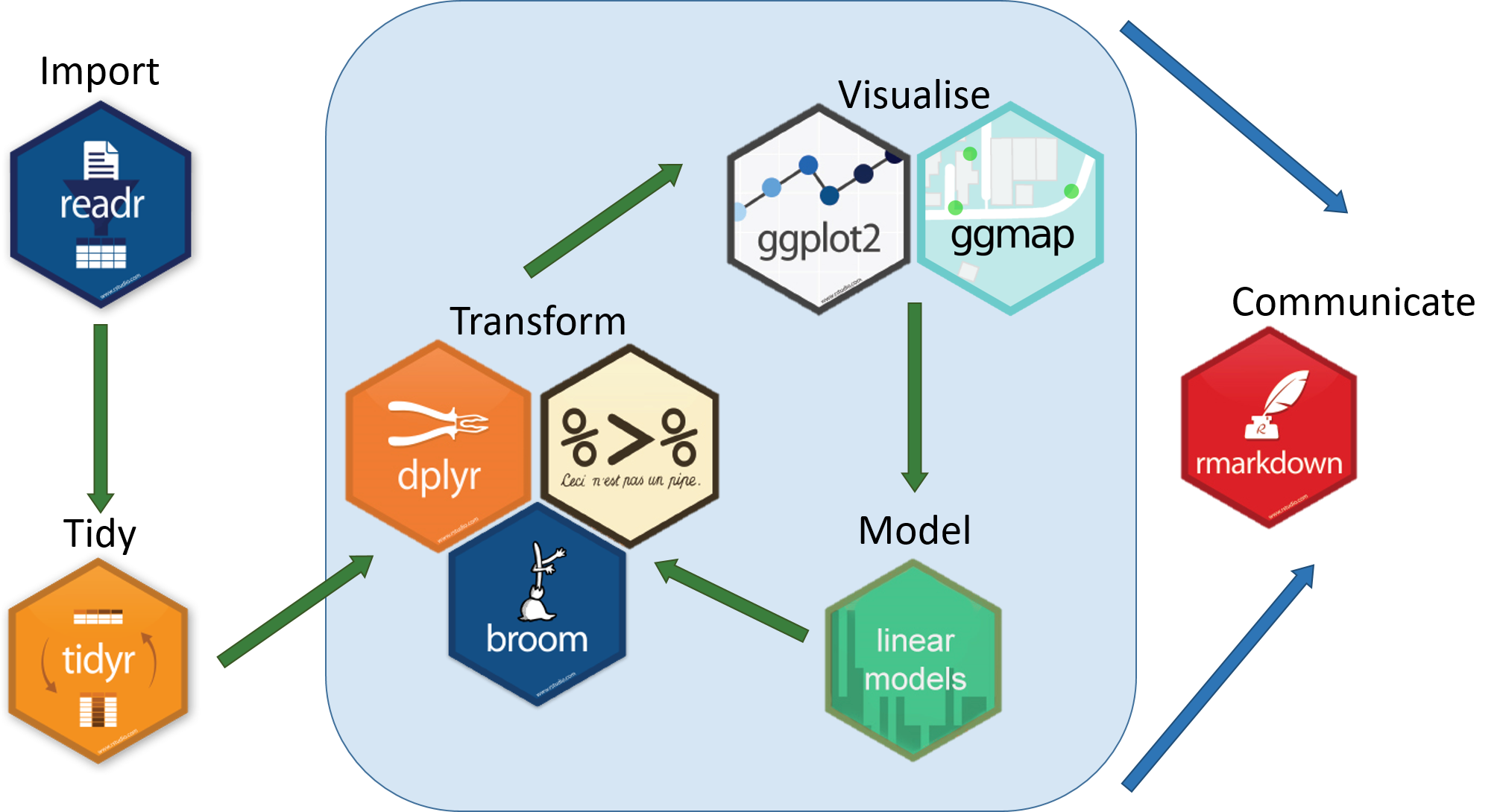Image Credit: Aberdeen Study Group

We are going to explore some of the basic features of the tidyverse using data from the gapminder project, which have been bundled into an R package. These data give various indicator variables for different countries around the world (life expectancy, population and Gross Domestic Product). We have saved these data as a .csv file called gapminder.csv in a sub-directory called raw_data/ to demonstrate how to import data into R.

Reading in data

Any .csv file can be imported into R by supplying the path to the file to readr function read_csv and assigning it to a new object to store the result. A useful sanity check is the file.exists function which will print TRUE is the file can be found in the working directory.

## This will print the current location of our working directory
getwd()

[1] "C:/work/personal_development/markdunning.github.com/training/r_part1"

gapminder_path <- "raw_data/gapminder.csv"
file.exists(gapminder_path)

[1] TRUE

The getwd(), and file.exists(...) functions have been used here as you may find them useful in your own work. If we are confident that we know where a file is located we can use read_csv as below.

Assuming the file can be found, we can use read_csv to import. Other functions can be used to read tab-delimited files (read_delim) or a generic read.table function. A data frame object is created.

library(readr)
gapminder_path <- "raw_data/gapminder.csv"
gapminder <- read_csv(gapminder_path)

Rows: 1704 Columns: 6
── Column specification ────────────────────────────────────────────────────────
Delimiter: ","
chr (2): country, continent
dbl (4): year, lifeExp, pop, gdpPercap

ℹ Use `spec()` to retrieve the full column specification for this data.
ℹ Specify the column types or set `show_col_types = FALSE` to quiet this message.

File paths

🤔

Why would specifying gapminder_path as Users/mark/Documents/workflows/workshops/r-crash-course/raw_data/gapminder.csv be a bad idea? Would you be able to re-run the analysis on another machine?

Reading from Excel (xls/xlsx) files

You can also read excel (.xls or .xlsx) files into R, but you will have to use the readxl package instead.

install.packages("readxl")
library(readxl)
## Replace PATH_TO_MY_XLS with the name of the file you want to read
data <- read_xls(PATH_TO_MY_XLS)
## Replace PATH_TO_MY_XLSX with the name of the file you want to read
data <- read_xlsx(PATH_TO_MY_XLSX)

If you get really stuck importing data, there is a File -> Import Dataset option that should guide you through the process. It will also show the corresponding R code that you can use in future.

The data frame object in R allows us to work with “tabular” data, like we might be used to dealing with in Excel, where our data can be thought of having rows and columns. The values in each column have to all be of the same type (i.e. all numbers or all text).

In Rstudio, you can view the contents of the data frame we have just created using function View(). This is useful for interactive exploration of the data, but not so useful for automation, scripting and analyses.

## Make sure that you use a capital letter V

View(gapminder)

# A tibble: 1,704 × 6
   country     continent  year lifeExp      pop gdpPercap
   <chr>       <chr>     <dbl>   <dbl>    <dbl>     <dbl>
 1 Afghanistan Asia       1952    28.8  8425333      779.
 2 Afghanistan Asia       1957    30.3  9240934      821.
 3 Afghanistan Asia       1962    32.0 10267083      853.
 4 Afghanistan Asia       1967    34.0 11537966      836.
 5 Afghanistan Asia       1972    36.1 13079460      740.
 6 Afghanistan Asia       1977    38.4 14880372      786.
 7 Afghanistan Asia       1982    39.9 12881816      978.
 8 Afghanistan Asia       1987    40.8 13867957      852.
 9 Afghanistan Asia       1992    41.7 16317921      649.
10 Afghanistan Asia       1997    41.8 22227415      635.
# ℹ 1,694 more rows

We should always check the data frame that we have created. Sometimes R will happily read data using an inappropriate function and create an object without raising an error. However, the data might be unusable. Consider:-

test <- read_table(gapminder_path)

── Column specification ────────────────────────────────────────────────────────
cols(
  `"country","continent","year","lifeExp","pop","gdpPercap"` = col_character()
)

Warning: 324 parsing failures.
row col  expected    actual                     file
145  -- 1 columns 3 columns 'raw_data/gapminder.csv'
146  -- 1 columns 3 columns 'raw_data/gapminder.csv'
147  -- 1 columns 3 columns 'raw_data/gapminder.csv'
148  -- 1 columns 3 columns 'raw_data/gapminder.csv'
149  -- 1 columns 3 columns 'raw_data/gapminder.csv'
... ... ......... ......... ........................
See problems(...) for more details.

View(test)

# A tibble: 1,704 × 1
   `"country","continent","year","lifeExp","pop","gdpPercap"` 
   <chr>                                                      
 1 "\"Afghanistan\",\"Asia\",1952,28.801,8425333,779.4453145" 
 2 "\"Afghanistan\",\"Asia\",1957,30.332,9240934,820.8530296" 
 3 "\"Afghanistan\",\"Asia\",1962,31.997,10267083,853.10071"  
 4 "\"Afghanistan\",\"Asia\",1967,34.02,11537966,836.1971382" 
 5 "\"Afghanistan\",\"Asia\",1972,36.088,13079460,739.9811058"
 6 "\"Afghanistan\",\"Asia\",1977,38.438,14880372,786.11336"  
 7 "\"Afghanistan\",\"Asia\",1982,39.854,12881816,978.0114388"
 8 "\"Afghanistan\",\"Asia\",1987,40.822,13867957,852.3959448"
 9 "\"Afghanistan\",\"Asia\",1992,41.674,16317921,649.3413952"
10 "\"Afghanistan\",\"Asia\",1997,41.763,22227415,635.341351" 
# ℹ 1,694 more rows

😬

The problem here is that we incorrectly told R that our file was “tab-delimited” rather than “comma-separated”. Tab-delimited means that a “tab” (four spaces) is used to distinguish the columns in the file. Therefore R cannot tell where the columns are, and the resulting data frame has a single column. R will not automatically use the appropriate read_csv or read_delim etc function, so you need to be careful

Quick sanity checks can also be performed by inspecting details in the environment tab. A useful check in RStudio is to use the head function, which prints the first 6 rows of the data frame to the screen.

head(gapminder)

# A tibble: 6 × 6
  country     continent  year lifeExp      pop gdpPercap
  <chr>       <chr>     <dbl>   <dbl>    <dbl>     <dbl>
1 Afghanistan Asia       1952    28.8  8425333      779.
2 Afghanistan Asia       1957    30.3  9240934      821.
3 Afghanistan Asia       1962    32.0 10267083      853.
4 Afghanistan Asia       1967    34.0 11537966      836.
5 Afghanistan Asia       1972    36.1 13079460      740.
6 Afghanistan Asia       1977    38.4 14880372      786.

We have used a nice, clean, dataset as our example for the workshop. Other datasets out in the wild might not be so ameanable for analysis in R. If your data look like this, you might have problems:-

We recommend the Data Carpentry materials on spreadsheet organisation for an overview of common pitfalls - and how to address them

• https://datacarpentry.org/spreadsheet-ecology-lesson/

Although R has many functions for data cleaning, if you are new to the language the best approach to such data would be to clean them before attempting to read into R.

Accessing data in columns

In the next section we will explore in more detail how to control the columns and rows from a data frame that are displayed in RStudio. For now, accessing all the observations from a particular column can be achieved by typing the $ symbol after the name of the data frame followed by the name of a column you are interested in.

RStudio is able to “tab-complete” the column name, so typing the following and pressing the TAB key will bring-up a list of possible columns. The contents of the column that you select are then printed to the screen.

gapminder$c

Rather than merely printing to the screen we can also create a variable

years <- gapminder$year

We can then use some of the functions we have seen before

min(years)

[1] 1952

max(years)

[1] 2007

median(years)

[1] 1979.5

Although we don’t have to save the values in the column as a variable first

min(gapminder$year)

[1] 1952

Coming next…

In Part 2 we will start to interrogate and visualise the data we have just imported

• Choosing which columns to show from the data
• Choosing what rows to keep in the data
• Adding / altering columns
• Sorting the rows in our data
• Introduction to plotting